W01 Using Indicator Variable (I) 非線性關係
2025-02-19三 14:10-17:00 林師模教授
| GoogleDoc-Note | Presentation | Paper/Report |
Review of basic statistics concept | A_Review_of_BasicStatistical_Concepts | 統計テスト | Prof.'s: Basic Probability Concepts |
預習: 參考 自習Econometrix and 變量分析 Multivariate Analysis | 五分鐘R語言系列第一集: 安裝下載及簡 | 閱讀筆記 Hackmd |
網頁: 統計學-自習 | Regression Analysis 回歸分析 | Research Methods預習 |
課本: 全文 Principles of Econometrics, 5th Edition | 參考資料查表(Statistical Tables和Formula Sheets) 等等 | EViews_prgprogram files |
By chapter:
Chp00|
Chp01|
Chp02|
Chp03|
Chp04|
Chp05|
Chp06|
Chp07|
Chp08|
Chp09|
Chp10|
Chp11|
Chp12|
Chp13|
Chp14|
Chp15|
Chp16|
Appendix|
GDoc_chp04 |
GDoc_chp05 |
查表: F-critical_value |
軟體: EViews | EViews Alternatives for Linux | 🎯 李宗璋老師Youtube的EViews教學 |
(I)練習: GoogleSheet-Exc#1 | Exc#2 |
(I)作業: Asig#1 | W08Asig#2 | W11Asig#3 | W14Asig#4 | W16 12/25 Asig#5-Final Report |
(II)作業: GoogleSheet- W15 05/28 Final Report 草稿 | Gimini-協助說明.pdf檔 |
W18 06/19四 應交出Final Report |
同學: 共有10人 主要是印尼,還有巴基斯坦和甘比亞同學
老師的講義 Ch-07 | 教科書內容 Chapter-07 |
Chp.7 非線性關係 Using Indicator Variables 和 Chp.8 異質變異 Heteroskedasticity 上學期沒講完,這期接著講,然後才講 Chp.9 動態模型、自我相關及預測 Regression with Time-Series Data: Stationary Variables
Final Report-老師會給sample format:
1.introduction
2.literature reivew related to your topic:
3.說明model 及estimation mothod will be used方法, explain what is data
4.最後emperical result跟conclusion
5.Reference. or Appendix (put data but not required)
- you can use any software you like, it generate the same result any way.
but you have to learn how to write your report professionaly. read good joural always.
今天講Chp7. Using Indicator Variables (I)
They are artificial variables that take on values of 0 or 1 to indicate the presence of absence of a "quality" or attribute.
下週講treatment對dummy variable的影響。
W02 Using Indicator Variable (II)
2025-02-26三 14:10-17:00 林師模教授
Reference:subject should study
7.1 Indicator Variables
今天講
7.2 Applying Indicator Variables
7.3 Log-Linear Models
7.5 Treatment Effects
將略過
7.4 The Linear Probability Model
7.6 Treatment Effects and Causal Modeling
回顧上週說的
Yi=B1 + B2Xi + ei
Pi=B1 + B2 Sqfti + ei
concern location which is a qualitative veriable
near university=1 not near=0
Pi=B1 + B2 Sqfti + B3 Li + ei
if L= 1 near or =0 not near; si we cab change model as:
Pi=B1 + B2 Sqfti + B3 Di + ei (D means dummy)
so
E(P|D=1) = B1 + B2 Sqfti + B3 = (B1+B3) + B2 Sqfti
E(P|D=0) = B1 + B2 Sqfti
This 2 model only different in intercept (B1, B1+B3), but same slope
B2
這稱為Basic Model 現在要開始展開:
1.因為slope相同 每增1 unit of sqft P 等比率增加。但如果在加個變數
sqftDi
Pi=B1 + B2 Sqfti + B3 Di + B4 (SqftDi) + ei
so
E(P|D=1) = B1 + B2 Sqfti + B3 = (B1+B3) + (B2+B4) Sqfti + ei
E(P|D=0) = B1 + B2 Sqfti
這樣不但intercept不同 slope斜率也會不同 (是否正還負 要看資料內容)
2.本週還要再加以擴大:請看Basic Model (D: near university=1 not
near=0)
Yi=B1 + B2Xi + ei 如果D反過來做 (D: near university=0 not near=1)
因為離大學近遠會影響 intecept 首先b3 就會變成負數;
其次intercept是基於距離大學近考慮起
Yi=(b1+b3_ + b2Xi -b3Di + ehat
E(Yi|Di=0)= (b1+b3) + b2Xi
E(Yi|Di=1)= (b1+b3) + b2*Xi -b3 b1 + b2Xi 想想看
3.我們來看例題p. EXAMPLE 7.1 The Universit Effect on House Price
先用utown跑eviews
在反過來設D 0 1 設變數 utown-1 這樣 0,1就反過來
再重跑equation
兩個estiamtion比較 就會看到 b1和B1 還有b2和B2相比的數字
以上說的是兩個dummy variable 還有0,1設定反過來的例子。
4.再想想這樣可以嗎 如果 LDi=1-Di
假設independent variable需要 ‘線性關係’ 這樣做會有collinearity問題,是不行的!
Yi=B1 + B2 Sqfti + B3 Di + B4 LDi + ei (這是perfect
collinearity所以不成立)
通常1個catogary只能有一個dummy,但如果有好幾個catogary的話,可以設多個dummy
老師有討論: 如果3個category(near,not near, far)你設為0,1,2 會怎樣:
restrcited result 只有 幾個B3的差別 不合理
如果用3個dummy 會有d1+d2+d3=1 的問題
請看 如果只用 兩個 就會可以有足夠的區別
所以知道 n個catergory就用n-1個dummy
如果有兩個qualitative 各有兩個catergory則2個dummy 就ok了
excel不管你有沒有colinearity 但eviews會提醒你
解決了:就是原來20250227-Vboxuser:變更密碼從22332587改為90922934lfh;(win10要用-eviews)
6.看(7.8)
WAGE=B1 +B2EDUC +d1BALACK +d2FENALE +g(BLACK*FEMALE) + e
看EXAMPLE 7.2 The Effects of Race and Sex on Wagep.323 跑eviews
因為是用non black=0 所以BLACK的coefficent 是負數,還有FEMALE也是負數
這是因為 WHITE MALE的dummy 都是設為0 做基數。
在這個例子: 所有差別都在intercept 而slope是一樣的,這叫: _______
7.再看看7.2.2 Qualitative Factors with Several Categories 上個小時已講過了。多個categories 只用 n-1個dummy veriables
再來看有趣的7.2.3 Testing the Equivalence of Two Regressions
(看老師畫的圖照相)
Pi=B1+ B2Si + ei 比如資料室這樣 中間有一段(比如小、大屋型)讓你覺得
如果跑兩個regression好像更接近事實, 但怎樣知道跑一個好 還是兩個好?
適或不適合 可以看 e hat square 的總和 SSE; 只要加上一個dummy veriable以區別兩組樣本 (d=0 or d=1)
這樣可以有兩個regression 再讓兩個regression的(sum sqare resid) SSE1+SEE2加總起來
這樣可以觀察 SSE-(SSE1+SSE2)的結果。 然而,怎樣設bundry以區分兩組data呢?
就要先設Hypothesis
H0: two regression is equvelant SSE=SSE1+SSE2
H1: not equal
所以設邊界 SSE-(SSE1+SSE2)/df1 / (SSE1+SSE2)/df2 =>F distribution
(F test)
SSE ~ χ^2^
以上是一種F test方法,而另一種方法就是用Dummy variable
Yi = B1 + B2Xi + B3Di + B4(Xi*Di) +ei
這個model 是不同intecept 和不同slope,這樣就是有兩條不同的regression line
這樣test可以設 H0: B3-B4 = 0
而如果B3 B4的 是significant 就可說 reject H0,則兩個regression line是不相等,是不同的
H1: B3 !=0 or B4!=0 or B3-B4!=0
老師再帶大家做F test (首先把用dummy variable做equation時的SSE 1919,862 先記好
然後開始做三個regression看看
- price c sqft; Sample: 1000; sum sqare resid= 1149512 (SSE)
- price c sqft; Sample: utown=1 (519); sum sqare resid= 123216.9 (SSE1)
- price c sqft; Sample: utown=0 (498); sum sqare resid= 113544.8 (SSE2)
SSE-(SSE1+SSE2)/df1 / (SSE1+SSE2)/df2 =>F
1149512-(123216.9+113544.8)/df1 / (123216.9+113544.8)/df2 =
df1 = (10000-2)-((519-2) + (481-2))=2
df2 = (519-2) + (481-2) = 996
算出和dummy一樣的結果
SSE-(SSE1+SSE2)/df1 / (SSE1+SSE2)/df2 =>F =1919,862
介紹: Chow Test: 是一種 Structure Break (看照片), 是有折線的意思。
其實Chow Tes 就是=SSE-(SSE1+SSE2)/df1 / (SSE1+SSE2)/df2 =>F
一樣的ideal也可用dummy vareable 結果是一樣但方法簡單多了,
看p.326: We might ask “Are there differences between the wage regressions for the south and for the rest of the country?” ……(7.10)
看.EXAMPLE 7.4 Testing the Equivalence of Two Regressions: The Chow Test
最後就是算出F value 0.6980 太小(老師找不到creitical value說應該是around 3) not reject the null hypothesis, coefficent basicly =0 this is called Chow Test.
這裡是把一個國家 分出了一個 南方,和非南方。 當這個時候,想知道會不會是個Structure breake. 因為reject the null hypothesis, coefficent basicly =0 所以我們知道DATA 沒有 Structure break (區分south 和不區分 沒有差別)
8.最後要講個p.332的 7.5 Treatment Effects
比如說:生病就須治療Treatment,從政府角度來說,就是推出一種policy。有時,想要先比較看看,政策改或不改變會有何差別,比如:基本工資調整,對就業率會有何影響?
舉例來說:如果你去醫院問人:你覺得健康比以前好嗎?這對來上月就來治療者或著剛來的病人顯然大有差別。剛來醫院就診的,就是覺得病得很,很不健康的嘛。因此,這樣的調查(抽樣)是一種selection bias因為 你選錯sample了,chosing wron sample,而最好的方法就是randomly select smple.
又舉例:調查學生覺得自己ecomometrics學得好不好?若此課程是required course就ok,但若是selectd course就會有selection bias. 顯然願意去選修此課的人,應是想要學好的人嘛。
本節講述如何用dummy verialbe來測出Treatment Effect,下週會從Treatment Effect繼續講!!
W03 Heteroskedasticity
2025-03-05三 14:10-17:00 林師模教授
老師的講義 Ch-07 | 教科書內容 Chapter-07 |
(p.332) [7.5] Treatment Effects
老師的講義 Ch-07 | 教科書內容 Chapter-08 |
關於Treatment effect 異質性Heterogeneity動畫說明
ATE: Average Treatment Effects 平均處理效應Average
treatment effect
-
對處理的隨機分配可確保在大量的實驗迭代中,分配給處理組的單位與分配給對照組的單位保持一致。
繼續看EXAMPLE 7.13 Estimating the Effect of a Minimum Wage Change:
Using Panel Data
解釋 ΔFTEi = β3 + δNJi + Δei (7.24) 的來由。
這到了panel data 的時候會解釋得更清楚,目前只研究兩個time periods。
到這裡chapter 7算講完了,沒講到的跳過去的,請你自己去研究。
注意: 本期的final report 可以參考這個Dummy
veriable來應用
hetero means different, if same we may say homo; so homoskedasticity
means same variance.
來介紹什麼是Hetroskedasticity:
Yi = B1 + B2Xi + ei 這是個simple linear regression
此時基本假設是
E(ei|Xi)=0 Var/(ei|Xi)=sigma square = contant = δ2
看 food.wf1
希望 flagerate around zero 但如果 不是的話, 就是有
Hetroskedasticity問題,也就是 ≠ δ2
Nature:varance is changing;
Consequences: 如果
太重要了!要記住 Var(b2) = δ2 / S(Xi-Xbar)2
這樣可以先算出Var(b2)應是個常數
但事實上 各個Xi可能會有異常的 e分佈 會有很多不同的δ2
,這樣的話還用OLS去算出的B2不正確
因為incorrect standard error所以 testing result 也會incorrect.
這是Hetroskedasticity問題! 也就是Consequences! 就是「testing will be not
correct」
回頭來看food.wf1 你可以看到Std. t-statastic 雖然都有數字,
但其實都是不正確的,
1.那麼怎樣判斷這有沒有Hetroskedasticity問題呢??
這種狀況是很普遍的,通常來自某些variable(有時只來自一兩個,但不一定,有時來自多個)
2.那麼怎樣判斷是那個變數促成這個Hetroskedasticity問題呢??
3.那麼怎樣解決這個Hetroskedasticity問題呢??
老師說: 這是不對的。都須要檢查
老師先教: 3.怎樣解決,才回頭教1,2. how to detect.
如果我們已經知道有Hetroskedasticity問題了。
1.有沒有其他正確的formula? 有些學者發展出一些formula:
請看Figure 8.1 這個問題。
這有個formula很複雜的:
var(b2|x)= σ2/∑Ni=1 (xi − x)2 (8.6)
p.374 (White heteroskedasticity-consistent estimator
(HCE)想出來的)
var⋀(b2)=[∑(xi − x)2]−1 {∑[(xi − x)2 ( NN − 2)ê2i]} [∑(xi − x)2]−1
(8.9)
用了這個var⋀(b2)就會more correct而testing value也就會更正確。
這就是White教授想出 consistent
estimator的方法。可以得到正確的SD,也稱作Robust Variance。
這是用原來的OLS但是另外去算出一個HCE
然而,既然有heteroskedasticity問題,光是估出HCE只解決e的問題,其實B2還是不正確。
(這時就要了解Gauss-Markov Theorem) 怎麼辦呢? OLS若要BLUE,best
linear/unbias 兩個可能有問題,需要確認或解決。 Should I do, and why I do
that?
如果沒有把握,可能要繼續用OLS但-如果我要換個方法來aprroach那我就要make assumption!
目前我現用food 案例來試著解決問題:
先算Robust Variance -estimate regression 時特的去選White
你會發現Std和t-value都變了
這是第一種option (看照片)
看 EXAMPLE 8.2 Robust Standard Errors in the Food Expenditure
Model
White Robust se: (p.374)
下週講 8.4 Generalized Least Squares: Known Form of
Variance
W04 Regression with time-series data: Stationary variables (I)
2025-03-12三 14:10-17:00 林師模教授
請假,去北海道!
W05 Regression with time-series data: Stationary variables (II)
2025-03-19三 14:10-17:00 林師模教授
運動會停課!
W06 Chp10- Random regressors & moment-based estimation (I)
2025-03-26三 14:10-17:00 林師模教授
老師的講義 Ch-09 | 教科書內容 Chapter-09 |
今天開始講第9章 Chapter 9 Regression with Time-Series Data:
Stationary Variables時間序列資料迴歸:平穩變量(定態變數)
- will skip 9.3 Forecasting and 9.5 Time-Series Regressions for Policy
Analysis 集中介紹 forcus on 0.1,2,4
- 2.另一種是autoregressive model 這是 an autoregressive process, is one where a varuable y depends on p ast balues of itself
-9.1 如果兩種 model並在一起就做autoregressive distributed lag model
公式為(9.3) 簡稱 ARDL(p,q)
-9.1.1 看書本421頁Infinite Distributed Lag Models (9.4)等解釋
這裡有個推導過程 一直到 (9.9) 本來有一堆infinite distribution number
被簡化到只剩兩個variable: yt-1 和 xt
這是來自(9.5)假設推導出來的
這是geometric dcline (figure9.3)的假設來的
- 這個model 也稱ARDL(1,0)
- infinite distributed lag(IDL) model
p.422討論An Autoregressive Error Model 接著p.423討論推導過程
在(9.4)兩邊乘上一個p 導到(9.15)變成有3個變數的公式,這就是ARDL(1,1) 公式That is, we have the constraint, or condition, β1 = −θβ0.
Autoregressive error models with more lags than one can also be transformed to special cases of ARDL models.
也就是說,我們有約束或條件β1 = −θβ0。滯後大於 1 的自迴歸誤差模型也可以轉換為特殊情況ARDL 模型。
p.4249.1.2 Autocorrelations
p1某一期間的 .. 見(9.17)
Testing the Significance of an Autocorrelation
用usmicro來做做看 figure 9.4
到19是significant (這裡沒秀出critical value) 但是你放大左邊圖 看有條虛線
是代表critical value 還有書上p.426有寫
The horizontal line drawn
at 2/√
173 = 0.121 is the significance bound for positive
Endogenous explanatory variables lead to biased OLS estimates. 使得β-hat不再是總體係數Beta無偏的、一致的估算值。
There are reasons why endogeneity occurs.
1.Omitted Variable Bias; 2.Reverse Causality; 3.Simultanueous Causality; 4.Endogenous Sample Selection遺留變量偏差(在家婦女沒被算進去). There are four estimation methods we often use to alleviate the endogeneity problem.
1.Instrumental Variables Estimation Method.
2.Panel Data Fixed Effects Methods.
3.Difference-In-Differences Approach.
4.Sample Selection Bias Correction.
autocorrelations.
根據staionary 的3個定義
variable has constant mean
variable has constant variance
covariance will depend on how many lag period apart for the data
point
可以來做判斷,是否為stationary
p.4279.2 Stationarity and Weak Dependence
判斷是否為stationaity 最終要根據chp12章教的unit rot tests方法
來判斷
Endogenous explanatory variables lead to biased OLS estimates. 使得β-hat不再是總體係數Beta無偏的、一致的估算值。
There are reasons why endogeneity occurs.
1.Omitted Variable Bias; 2.Reverse Causality; 3.Simultanueous Causality; 4.Endogenous Sample Selection遺留變量偏差(在家婦女沒被算進去). There are four estimation methods we often use to alleviate the endogeneity problem.
1.Instrumental Variables Estimation Method.
2.Panel Data Fixed Effects Methods.
3.Difference-In-Differences Approach.
4.Sample Selection Bias Correction.
Eviews檔案usmacro的 inf是inflation rate, u 是unemployee rate, g是gdp growth rate, c是constant,
台灣的unemployee rate 約是3.多
9.4 Testing for Serially Correlated Errors
理論上e是沒有
但實際上存在的 當我們estimate後應當test一下 有沒有Correlated Errors
這兒有個公式可檢查(9.45)
看EXAMPLE 9.10 看圖只有3個超出 cretical value 所以他說It is reasonable to conclude that there is no strong evidence of serial correlation.
estimate equation:
先做 u c u(-1) u(-2) g(-1) 再去看residule
接著做 u c u(-1) g(-1) 再去看residule
9.4.2 Lagrange Multiplier Test - formal test
可以run (9.47) 可以得到一個rough result
但通常不用這樣做,而是去做formal test 就是去
(9.49)這公式的depnet是residule
跑這個equation叫做Lagrange Multiplier Test 注意看他的Ho是p=0
這是測autoregression error
注意 有幾個period就有幾個df
EXAMPLE 9.12
ARDL(1,1) model
你看那個ARDL(2,1)的p-value order 1,4可能not significant但2,3是significant
9.4.3 Durbin-Watson Test現在已很少用了 因為只能用在order 1 serials regression model
老師要跳過去section 5,但還有點時間,所以要講:
9.5.2 HAC Standard Erros
這個跟heterocedasticity很像,檢查residule
公式很複雜不用管,注意EXAMPLE 9.14 A Phillips Curve
經濟學上應該要學過Phillips Curve 菲利浦曲線 公式(9.64)
解釋了菲利浦曲線(英語:Phillips
Curve),紐西蘭統計學家威廉·菲利浦於1958年根據英國近百年(1861-1957)的總體經濟數據,畫出來的
菲利浦曲線
用philips5_aus.wf1
robust standard error
用inf c du DU Coefficient -0.398670
HAC
0.287846 這就是robust standard error
看TABKE 9.9
如果你有serious correlation 在你的model (像heterocedasticity 的GLS )
下週結束chp9, 開始10.
🎯Australia孫老師BX2122講得和林師模老師一樣的內容。可作複習用。今天複習
BX2122/EC5216 Topic 9-1 Regression with Time Series Data: Stationary Variable再看
BX2122/EC5216 Topic 9-2 Regression with Time Series Data: Stationary Variable
中文部份看了:
中原國貿系yang powebe楊奕農TSA ch1.1a 假性迴歸有繁體字幕8m
? 一階自我相關(AR模型)
? 需求法則 價格與需求成反向變動 P=SP*
TSA ch1.1b 從AR(1)模型談起20m 數據的前世今生Auto
Rregressive模型,自我相關(你過去怎樣,未來會不會怎樣),AR(1)1代表落後1期的意思。
Yt=f(Yt-1) Yt=Φ1 Yt-1 (AR線性關係/目前已發展到可計算非線性關係了)
- 遞迴推算solutionn by interation之規則
- 遞迴推算規則之一般式 Yt=(Φ1) Yt-1
只要知道第一期,就可推導出各期。=> 16:00推導yt=(a1)^t y0;
TSA ch1.1c 包含截距項的AR(1)模型(12m/有字幕-v24a)
- 等比級數,等加級數公式。
TSA ch1.3~1.4 蛛網理論+收歛值和經濟長期均衡8m蛛網理論 reduce form: Pt=a0
+ a1 Pt-1
- 定態意指「長期均衡」。有意義的均衡=不是泡沫化。 |a1|<=1
staionarity定態
TSA ch.1.5a 加入誤差觀念的 AR(1) 模型 16m v23b
- 「些許」誤差長期平均而言應該會,「相互抵銷mutual offset」 即E(ut)=0
for all t.
W07 Chp10-Endogenous Regressors and Moment-Based Estimation
隨機解釋變數和動差估計
2025-04-02三 14:10-17:00 林師模教授
老師的講義 Ch-09 | 教科書內容 Chapter-09 |
老師的講義 Ch-10 | 教科書內容 Chapter-10 |
本週要結束chp9, 開始10.
Autoregressive (AR):自我迴歸部分,表示當前值是過去值的線性組合。
Moving Average(MA):滑動平均部分,表示誤差項是當前及過去誤差項的線性組合。
ARMA 模型通常以 ARMA(p, q) 表示,其中
p 是自我迴歸項的數量
q 是滑動平均項的數量
現在要接著講9.5.3. Estimaton with AR(1) Errors
看p.453 (相片有9.14) 用9.12 代入 導出 9.15
有兩個方法來estimatte這個model
1.一個是noliear (就是這個9.68)
2.另一個可以do some manipulation操縱 這就是(9.70)我要教的 section:9.5
那9.70 就可以做OLS但是 要先對 9.69進行處理。但這個方法 需要先estimate出p來
方法在p.454 e Cochrane–Orcutt estimator. (其實這就是GLS)
看EXAMPLE 9.15 The Phillips Curve with AR(1) Errors
equation: inf c du equation: nonlinean:
inf=c(1)(1-c(2))+c(2)inf(-1)+c(3)du-c(2)c(3)*du(-1)
要換到第10章了,今天只講section 1,2
請舉例說明,什麼是Endogenous Regressors
當Xt不是random時 原來的strict exogeneity assumption嚴格外生性假設, E(ei|xi)=0
但是如果xt是 random時 特別是small samples時(<30)
但在real world有時是large sample 照說會比較容易達到strict
exogeneity
但
根據Gauss-Markov therem 當條件都符合時 OLS > BLUE
when we asuume the xt is random
放棄第一個assumption 保持其他兩個
以上這些 要去詳閱Chp10的課文(找strict exogeneity上下文)p.482
10.1.3 Proving the Inconsistency of OLS
W08 Chp11- Simultaneous equations models
2025-04-09三 14:10-17:00 林師模教授
Reference:subject should study
supply curve and demand curve; 跟6,7週的觀念很相近
老師的講義 Ch-10 | 教科書內容 Chapter-10 |
老師的講義 Ch-11 | 教科書內容 Chapter-11 |
2025/04/09三
Simultaneous Equations Models 聯立方程式模型
國語五分鐘計量經濟學 【Mandarin國語】五分鐘計量經濟學(計量經濟學輔導)第二十三集:多元變量模型OLS估計量什麼時候跟部分模型OLS估計量相同?
【Mandarin國語】五分鐘計量經濟學(計量經濟學輔導)第二十四集:什麼是矩陣的基礎概念和特點?
Solutions to Problems 1-4 (Chapter 16 Simultaneous Equations Models) | Introductory Econometrics 75
Simultaneous equation models - an introduction p.487 況
上週複習
p.487 10.2Cases in Which x and e are
Contemporaneously Correlated x 和 e 同時相關的情況
這就叫endogenous.內生問題. 這節解釋原因,像Measurement Error, 像(10.1)
理論公式原是permenet income但現實世界的資料,只能有corrent
income,然而這兩者是不同的,(10.2)就是講怎樣利用current
income去代用,重新 rearrange equation. (10.3)
如此一來,公式(10.4)就會看到 cov(Xi, ei) ≠ 0 表示,其實Xi 和 ei
是相關corelated的。 這是第一個問題: Measurement Error problem.
另個問題是10.2.2 Simultaneous Equations Bias 聯立方程式偏差
解釋(10.5)Q P e 之間都會互相影響,如果這裡用OLS就會有biased, 因為P
有endougenous問題。 這就是一種Simultaneous Equations Bias
聯立方程式偏差
p.489 10.2.3 Lagged-Dependent Variable Models with Serial
Correlation 具有序列相關的滯後因變數模型
t-1和t 前後會有相關。
et會受et-1影響,Yt-1也可能受et-1影響。
你看這幾個公式,前後的independent variables 和error
tern都會相互影響。
p.489 10.2.4 Omitted Variables 省略的變數
(10.6) 像ei
可能包括有影響力的比如ability,但ability難衡量,就被括進ei了,這就是個omitted
variables。可能造成EDUC 成了endougenous.
EXAMPLE 10.1 Least Squares Estimation of a Wage Equation
-老師有解釋 wage和educ 關係
Endogenous explanatory variables lead to biased OLS estimates. 使得β-hat不再是總體係數Beta無偏的、一致的估算值。
There are reasons why endogeneity occurs.
1.Omitted Variable Bias; 2.Reverse Causality; 3.Simultanueous Causality; 4.Endogenous Sample Selection遺留變量偏差(在家婦女沒被算進去). There are four estimation methods we often use to alleviate the endogeneity problem.
1.Instrumental Variables Estimation Method. 工具變量法 IV
2.Panel Data Fixed Effects Methods. 固定效應模型 FE
3.Difference-In-Differences Approach. 差分法 DiD
4.Sample Selection Bias Correction.樣本選擇偏差校正法
第4也有另一種: 配對法Matching Methods,和 樣本選擇偏差校正法Sample Selection Bias Correction不一樣。
解釋endogeneity 內生性
When an explanatory variable is
contemporaneously correlated with the regression error one is said to
have an “endogeneity problem.”
當解釋變數與迴歸誤差同時相關時,就稱為存在「內生性問題」。
(可以看Backup▼2 自習課程2.Bob-19集的說明:什麼是內生解釋變量和外生解釋變量?)
今天開始教Moment-Based Estimation
首先:
p.482 strict exogeneity
Xi is nonstochastic
E(ei)=0 E(Xi
ei)=0 cov(Xi, ei)=0 這是三個基本的假設。 但在小樣本時,因為ei是random
所以 cov(Xi, ei)=0 這假設可能無法成立,滿足。
所以要放鬆限制,只保留這兩個假設: E(ei)=0 且 E(Xi ei)=0
這就是為符合strict exogeneity 所進行的改變slightly change。
其次:
如果ei 是random 那麼做OLS estimate會有biased 因為ei和X
會有corelated
這就是一種endorenous 也就是cov(Xi, ei) ≠ 0
那麼怎樣找出一個unbiased 的方法呢 對大樣本做estimation
methond時可以找到很接近真實的parameter這叫consistent 。
我們需要做test來看看有沒有這樣的biased 所以今天要教: 怎樣解決biased
跟怎樣檢查test
p.490 10.3 Estimators Based on the Method of
Moments基於矩法的估計量
花了一小時複習,現在重頭戲才要開始!
p.490 10.3.1 Method of Moments Estimation of a Population Mean and
Variance總體平均數和變異數的矩估計法
Kth momnet of Y
注意Population moment和sample moment
推導到(10.8) 然後看例子(10.9)=the second moment of Y-square(first monent
of Y)
這樣又可以推導到(10.12) 但這是給population的,按統計學所教sample應是/N-1
然而,因這是large sample random出來所以差別不大,所以直接就用N了。
p.491 10.3.2 Method of Moments Estimation in the Simple Regression
Model簡單迴歸模型中的矩估計法
這是第一種方法: 用兩個假設(10.13)(10.14)為基礎 代換後,解聯立方程式。 解出答案來 b1=ybar - b2 xbar
在這裡show出了moment的好用!!
p.492 10.3.3 Instrumental Variables Estimation in the Simple
Regression Model簡單迴歸模型中的工具變數估計
這是第二種方法:
無中生有來個Z (以取代X) 做工具
1.這個Zi一定不該對Y有影響(不然他就是independent variable了)
2.cov(Zi, ei)=0
3.Zi應該highly corelated with Xi - 像那個EDUC例子 取代的可能是 mother’s or fater’s or both EDUC,
- 如果拿mother’s EDUC雖不完美,但可以作為Instrumental
Variables來estimation. 這樣就會生出(10.15)的替代公式來了
注意(10,17)和10.3.2推導出的有所不同,然而計算出的結果是一樣(相當一致)的。
p.493 10.3.4 The Importance of Using Strong
Instruments使用強大儀器的重要性
p.494 10.3.5 Proving the Consistency of the IV
Estimator證明IV估計量的一致性
p.495 EXAMPLE 10.2 IV Estimation of a Simple Wage
Equation簡單工資方程式的估計
這是利用(10.17)的公式去算出的,用了這個以後,原來的EDUC影響力,減至0.0385了
用Eviews跑跑看mroz 注意 estimation時 要加條件 先做一次
在換成instrument 在eviews要用 two stages estimate;
p.495 10.3.6 IV Estimation Using Two-Stage Least Squares
(2SLS)使用兩階段最小平方法(2SLS)「二階動差法」進行 IV 估計
用two
stage法結果是和instrument一樣的
你可以用EXAMPLE 10.3 2SLS Estimation of a Simple Wage
Equation來練習看看
這個eviews做出來的,只會給你第二stage也是最終的結果,過程的first
stage就不會秀出(也不重要)了
p.49 10.3.7 Using Surplus Moment
Conditions利用剩餘力矩條件
可以用媽媽的EDUC也可以用爸爸的EDUC,甚至兩個都用,這樣可以有好幾個equations
那麼怎樣把他合併起來呢,這方法就叫做Surplus Moment
注意看eviews的相片,在instrument那裡 放了兩個變項mother father
p.498 10.3.8 Instrumental Variables Estimation in the Multiple
Regression Model多元迴歸中的工具變數估計迴歸模型
請看相片,estimate: log(awge) c educ exper exper^2 加上了exper
exper^2
那麼instruent: mothereduc fathereduc exper exper^2 就也要加上exper
exper^2
下次上課講很重要的: 如何對算出來的結果 做test! 然後Chapter 10就結束了。
W09 (期中考)
2025-04-16三 14:10-17:00 林師模教授
考試週休假不上課!
W10 Regression with time series data: Nonstationary variables (I)
2025-04-23三 14:10-17:00 林師模教授
老師的講義 Ch-10 | 教科書內容 Chapter-10 |
老師的講義 Ch-11 | 教科書內容 Chapter-11 |
p.498 10.3.8 Instrumental Variables Estimation in the Multiple Regression Model
兩個stage 二階動差法。用EXAMPLE 10.5再解釋一遍
看Table 10.1 的MOTH FATH 的p都是0 所以是good! significant!
還學了10.3.9 Assessing Instrument Strength Using the First-Stage Model
p.503 10.3.10 Instrumental Variables Estimation in a General
Model
你看p,503 的(10.28) 的Good 和 Bad variables.
看下面還有L = lucky variables 如果just-identified是OK,
即使是over也沒關係!
用GMM可以調整原來的model讓
the GMM estimator has smaller variances than the IV estimator in large samples.
美國教科書 稍難但更重要 William Greene (2018) Econometric Analysis, Eighth Edition,Pearson Prentice-Hall, Chapter 13. 本書不講GMM 你可看此書去學!
接著開始講: p.506 10.4.1 The Hausman Test for Endogeneity
如果只有一個 ex=ndogenous variable只要步驟1,2 若多個要再做3.
跑Eviews試試看 EXAMPLE 10.7 Specification Tests for the Wage
Equation
這是做步驟1,2的。
20250423 Vboxuser已變更密碼為: 22332587lfh
1.run model: educ c exper exper^2 mothereduc fathereduc
sample if lfp=1
看相片 generate series by equation vhat
2.run model: lab(wage) c educ expr exper^2 vhat
sample if lfp=1
參考Table 10.2 核對vhat 的Prob.
現在想第2步model Eviews跑stability diagonostics>Hausman test
試試看
EViews 是可以直接做 Hausman
检验的,且操作相对简单,适合面板数据模型选择的统计检验需求。
老師忘了怎做,須自己學習。
第11章Simultaneous Equation Model 引用了重要的第10章的觀念
11.1 A Supply and Demand Model
(equilibrium 平衡 )
看Fugyre 11.3 P Q 是endougenous variable
要解這個 就先要學會11.2 The Reduced-Form Equations
Structural
equation 和 Reduced-form equation 的不同是
Structural equation 是based specify by theory; (right可能有endougenous
varialbe)
而 only have endougenous varialbe in left hand side and no one in right
side.
經過manipulation 讓右邊沒有endougenous variable 才可以有consistent
estimation
有了reduced-form (11.4) (11.5)就可以do OLS estimation
11.3 Failue 跳過去,你可以自己看。
11.4 The Identification Problem 這個比較重要
看EXAMPLE
11.1 Supply and Demand for Truffles 松露
首先就是先要確定 是不是可以identified
一階動差 first stage 其實就是 reduced form equation
下週(4/30)要講這個,很有趣的例子! EXAMPLE 11.2 Supply and Demand
at the Fulton Fish Market
W11 Regression with time series data: Nonstationary variables (II)
2025-04-30三 14:10-17:00 林師模教授
老師的講義 Ch-11 | 教科書內容 Chapter-11 |
老師的講義 Ch-12 | 教科書內容 Chapter-12 |
LibreOffice的獨立樣本t檢定公式在哪裡? 碩博士生進行論文研究前,請先搞懂這四個“假設”!
每天都有supply 和demand兩股力量在角力,這是個聯立方程式。
可以找出這兩條線的關係嗎!
fultonfish 檔案; 每週只有5天資料; 所以dummy varible只要設4個; (11.13) 把QUAN 和PRICE做log nature
(11.14)如果前三天有壞天氣 STORMY=1 不是壞天氣就是=0;
The Fulton Fish Market has operated in New York City for over 150
years. The prices for fish are determined daily by the forces of supply
and demand. Kathryn Graddy2 collected daily data on the price of whiting
(a common type of fish), quantities sold, and weather conditions during
the period December 2, 1991, to May 8, 1992. These data are in the file
fultonfish.
富爾頓魚市在紐約市已經經營了 150 多年。魚的價格每天由供需關係決定。 Kathryn Graddy2 收集了 1991 年 12 月 2 日至 1992 年 5 月 8日期間牙鱈(一種常見的魚類)的價格、銷售數量和天氣狀況的每日數據。這些資料保存在fultonfish 檔案中。
Fresh fish arrive at the market about midnight. The wholesalers, or
dealers, sell to buyers for retail shops and restaurants. The first
interesting feature of this example is to consider whether prices and
quantities are simultaneously determined by supply and demand at all.3
We might consider this a market with a fixed, perfectly inelastic
supply.
新鮮的魚大約在午夜抵達市場。批發商或經銷商將產品銷售給零售店和餐廳的買家。這個例子的第一個有趣的特點是考慮價格和數量是否同時由供給和需求決定。
3 我們可以認為這是一個具有固定的、完全無彈性供給的市場。
At the start of the day, when the market is opened, the supply of
fish available for the day is fixed. If supply is fixed, with a vertical
supply curve, then price is demand-determined, with higher demand
leading to higher prices but no increase in the quantity supplied. If
this is true, then the feedback between prices and quantities is
eliminated. Such models are said to be recursive and the demand equation
can be estimated by OLS rather than the more complicated two-stage least
squares procedure.
每天一開始,當市場開放時,當天的魚的供應量是固定的。如果供給量固定,且供給曲線為垂直,則價格由需求決定,需求增加會導致價格上漲,但供給量不會增加。如果這是真的,那麼價格和數量之間的回饋就會被消除。據稱,此類模型是遞歸的,需求方程式可以透過
OLS 來估計,而不是更複雜的兩階段最小二乘程序。
However whiting fish can be kept for several days before going bad,
and dealers can decide to sell less, and add to their inventory, or
buffer stock, if the price is judged too low, in hope for better prices
the next day.
然而,鱈魚可以保存幾天才會變質,如果價格被判斷為過低,經銷商可以決定減少銷售量,並增加庫存或緩衝庫存,
希望第二天的價格更優惠。
Or, if the price is unusually high on a given day, then sellers can
increase the day’s catch with additional fish from their buffer stock.
Thus despite the perishable nature of the product, and the daily
resupply of fresh fish, daily price is simultaneously determined by
supply and demand forces. The key point here is that “simultaneity” does
not require that events occur at a simultaneous moment in time.
或者,如果某一天的價格異常高,那麼賣家可以從緩衝庫存中增加魚的數量。因此,儘管產品易腐爛,每天都會補給新鮮魚,但每日價格還是由供需力量同時決定。這裡的關鍵點是「同時性」並不要求事件在時間的同一時刻發生。
Let us specify the demand equation for this market as where QUANt is
the quantity sold, in pounds, and PRICEt is the average daily price per
pound. Note that we are using the subscript “t” to index observations
for this relationship because of the time series nature of the data. The
remaining variables are indicator variables for the days of the week,
with Friday being omitted. The coefficient α2 is the price elasticity of
demand, which we expect to be negative. The daily indicator variables
capture day-to-day shifts in demand. The supply equation is
讓我們指定該市場的需求方程,其中 QUANt 是銷售數量(以磅為單位),PRICEt
是每磅的每日平均價格。請注意,由於資料的時間序列性質,我們使用下標“t”來索引這種關係的觀察結果。其餘變數是星期幾的指示變量,但星期五省略。係數α2是需求價格彈性,我們預期係數為負。每日指標變數捕捉需求的日常變化。供給方程式是
The coefficient β2 is the price elasticity of supply. The variable
STORMY is an indicator variable indicating stormy weather during the
previous three days. This variable is important in the supply equation
because stormy weather makes fishing more difficult, reducing the supply
of fish brought to market.
係數β2是供給價格彈性。變數 STORMY是一個指示變量,表示前三天的暴風雨天氣。這個變數在供應方程中很重要,因為暴風雨天氣使捕魚更加困難,從而減少了進入市場的魚的供應。
老師平常用***可計算一般均衡模型(Computable General EquilibriumModel,. 以下簡稱CGE 模型)
如果change=1 表示lage inventory 如果是0 那共給曲線是fixed 是垂直的
你看 若是作Supply (11.14)出來的結果(還是讓你跑出來) p都是insignificant 不能用! 這是因為coleairatlity 只能是作Demand estiamtion就可以!
看excesise 11.25
Reconsider Example 11.2 on the supply and
demand for fish at the Fulton Fish Market. The data are in the file
fultonfish. In this exercise, we explore the behavior of the market on
days in which changes in fish inventories are large relative to those
days on which inventory changes are small. Graddy and Kennedy (2006)
anticipate that prices and quantities will demonstrate simultaneity on
days with large changes in inventories, as these are days when sellers
are demonstrating their responsiveness to prices. On days when inventory
changes are small, the anticipation is that feedback between prices and
quantities is broken, and simultaneity is no longer an issue.
重新考慮例 11.2 中富爾頓魚市的魚類供需。資料位於檔案 fultonfish中。在本練習中,我們探索魚類庫存變化較大的日子相對於庫存變化較小的日子的市場行為。Graddy 和 Kennedy (2006)預計,在庫存發生較大變化的日子裡,價格和數量將表現出同時性,因為這些日子裡賣家正在表現出對價格的反應能力。在庫存變化較小的日子裡,預計價格和數量之間的回饋會被打破,同時性不再是問題。
b.Obtain the OLS residuals v̂t2 from the reduced-form equation
estimated in (a). Carry out a Hausman test, as discussed in Section
10.4.1, for the endogeneity of ln(PRICE) by adding v̂t2 11.6 Exercises
555 as an extra variable to the demand equation in (11.13), estimating
the resulting model by OLS, and testing the significance of v̂t2 using a
standard t-test. If v̂t2 is a significant variable in this augmented
regression then we may conclude that ln(PRICE) is endogenous. Based on
this test, what do you conclude?
從 (a) 估計的簡化形式方程式中取得 OLS 殘差 v̂t2。按照第 10.4.1
節中的討論,通過將 v̂t2 11.6 練習 555 作為額外變量添加到 (11.13)
中的需求方程,通過 OLS 估計得到的模型,並使用標準 t 檢驗來檢驗 v̂t2
的顯著性,對 ln(PRICE) 的內生性進行豪斯曼檢驗。如果 v̂t2
是這個增強迴歸中的一個顯著變量,那麼我們可以得出結論,ln(PRICE)
是內生的。根據此測試,您得出什麼結論?
看照片 自己做一個vhat 來estimate
c.Estimate the demand
equation using two-stage least squares and OLS using the data when
CHANGE = 1, and discuss these estimates. Compare them to the estimates
in Table 11.5.
使用 CHANGE = 1 時的數據,利用二階段最小平方法和 OLS
估計需求方程,並討論這些估計值。將它們與表 11.5 中的估計值進行比較。
d.insignificant
e.
f.
第10章學會內生和外生變數 第11章學會用工具變數 和二乘法
現在來談第12章
CHAPTER 12 Regression with Time-Series Data: Nonstationary
Variables
stationary variable的定義? 要有constant
mean而不是越來越大或越來越小
如果yt=a +b t^2 是個codragtic line 做一次微分會變成lienean line=
nonestationary,
再一次 才會變成 stationary
fracurate
12.1.1 Trend Stationary Variables
stochastic trend –deterministic trend
下週開始講這個12.1.2 The First-Order Autoregressive Model 一階自迴歸模型 (中文課本p.516)
Chpt.14講完後,會規定期末報告題目 因所有time serieals都講完了.接下來講panal data model
W12 Chp13- Vector error correction and vector autoregressive models (I)
2025-05-07三 14:10-17:00 林師模教授
老師的講義 Ch-12 | 教科書內容 Chapter-12 |
Youtube一階自迴歸模型-楊P TSA ch1.1b 從AR(1)模型談起 20m
-楊亦農P TSA ch1.1a 假性迴歸 一開始就要檢測變數是不是全部定態stationality,只要一個不是就會出現假性迴歸。 白噪音就是古典回歸的殘差。 (若看p value拒絕虛無假設,意味x和y有關係)
-楊亦農P TSA ch1.1b 從AR(1)模型談起 20m
-楊亦農P TSA ch1.1c 包含截距項的AR(1)模型
-楊亦農P TSA ch1.3~1.4 蛛網理論+收歛值和經濟長期均衡 (8m)
p.570 12.1.2 The First-Order Autoregressive Model
univariate 單變數 等比級數Geometric series
“shocks” or “innovations.” 「衝擊」還是「創新」。
drift漂移 digress離題 首先要區分 stationary or nonstationary variable
-
stationary 和 non-stationary variable 的定義與如何區分
- 在時間序列分析中,定態 (Stationary) 和 非定態 (Nonstationary) 是非常重要的概念,它們描述了時間序列的統計性質是否隨時間變化而改變。
1. 定態變數 (Stationary Variable) 或 定態時間序列 (Stationary Time Series)
一個時間序列 Xt 被稱為是定態的,如果其統計特性(如均值、變異數和自相關)不隨時間而變化。
更精確地說,我們通常關注的是弱定態 (Weak Stationarity) 或 協方差定態 (Covariance Stationarity)。一個時間序列 Xt 如果滿足以下三個條件,則稱為弱定態: - 均值是常數 (Constant Mean): 對於所有的 t,期望值 E[Xt]=μ,其中 μ 是一個常數。
- 變異數是常數 (Constant Variance): 對於所有的 t,變異數 Var[Xt]=σ2,其中 σ2 是一個常數。
- 自協方差僅取決於時間間隔 (Autocovariance Depends Only on Lag): 對於任何時間點 t 和任何間隔 k,Cov[Xt,Xt−k]=γk,其中 γk 僅取決於間隔 k,而不取決於具體的時間點 t。
簡單來說,定態序列在不同的時間段內看起來是相似的,沒有明顯的趨勢、週期性(除了固定頻率的週期)或隨時間變化的波動。
2. 非定態變數 (Nonstationary Variable) 或 非定態時間序列 (Nonstationary Time Series)
一個時間序列 Xt 被稱為是非定態的,如果它不滿足定態的任何一個或多個條件。
常見的非定態來源包括: - 趨勢 (Trend): 均值隨時間系統性地增加或減少(如經濟增長數據)。
- 季節性 (Seasonality): 具有固定的週期性模式(如每月或每季的銷售數據)。雖然有些定義認為嚴格的季節性可能導致非定態,但很多時候季節性可以通過差分或虛擬變數處理後視為(經調整的)定態。
- 隨時間變化的變異數 (Time-varying Variance): 序列的波動性隨時間變化(稱為異質變異數,Heteroskedasticity)。
- 隨時間變化的自相關結構 (Time-varying Autocovariance): 序列與自身過去值的相關性結構隨時間變化。
- 單位根 (Unit Root): 這是一種特殊的非定態形式,常見於隨機漫步 (Random Walk) 等過程。具有單位根的序列其過去的震盪會持續影響未來值,導致變異數隨時間增加,並且衝擊是永久性的。
非定態序列的統計特性是隨時間變化的,不同時間段的數據可能看起來非常不同。
3. 如何區分這兩者?
區分定態和非定態變數通常結合使用圖形分析和統計檢定:
圖形分析 (Graphical Analysis): - 繪製時間序列圖 (Plot the time series): 觀察數據是否有明顯的趨勢、季節性或隨時間變化的變異數。定態序列通常會圍繞一個常數均值上下波動。非定態序列則可能向上或向下移動,波動幅度可能變大或變小。
- 繪製自相關函數 (ACF) 和偏自相關函數 (PACF) 圖 (Plot the Autocorrelation Function and Partial Autocorrelation Function):
- 定態序列: ACF 會相對快速地衰減到零(可能是指數衰減或震盪衰減)。PACF 可能在某個滯後處突然截斷或也快速衰減。
- 非定態序列 (特別是具有單位根的): ACF 會非常緩慢地衰減到零,甚至長時間保持較高的值(通常呈線性緩慢衰減)。這是因為序列的趨勢或單位根導致遠期的觀測值之間仍然高度相關。PACF 可能在第一個滯後處有顯著的尖峰。
- 這是區分定態和非定態最常用的方法。這些檢定旨在判斷序列是否具有單位根,因為單位根是非定態的一個常見原因。
- 擴展迪基-福勒檢定 (Augmented Dickey-Fuller, ADF Test):
- 虛無假設 (H0):時間序列是非定態的(存在單位根)。
- 對立假設 (H1):時間序列是定態的。
- 如果檢定統計量小於臨界值(通常在負數區域),我們拒絕 H0,認為序列是定態的。否則,我們無法拒絕 H0,認為序列是非定態的。
- Phillips-Perron (PP) 檢定: 與ADF類似,也檢定單位根,但對異質變異數和序列相關更為穩健。
- Kwiatkowski-Phillips-Schmidt-Shin (KPSS) 檢定:
- 虛無假設 (H0):時間序列是定態的。
- 對立假設 (H1):時間序列是非定態的。
- 與ADF/PP相反,如果檢定統計量大於臨界值,我們拒絕 H0,認為序列是非定態的。
通常在實務上,我們會同時使用圖形分析和統計檢定來判斷時間序列的定態性。如果發現序列是非定態的,通常需要對其進行轉換(如取對數、差分等)使其變成定態序列,以便應用基於定態假設的時間序列模型(如 ARIMA 模型)。
如果 ρ>1 會越來越大到爆炸 所以是nonstaionary variable
p.571 左上的(a) yt=0.7yt–1 + vt 因為mean=0 variance
是constant所以是stationary variable 是stationary
(12.13) 如果是non zero mean! 如果是1的話,會產生 3.33的倍數的
看圖 (b) yt = 1 + 0.7yt–1 + vt 因為有了截距是1 mean不再是0
變成3.33
是stationary
看圖 (c) yt = 1+ 0.01t + 0.7yt–1 + vt 這是第三種 有趨勢的model
第四種請看 (d) yt = yt–1 + vt 不符合constant mean 和variance所以是nonstationary 這種模式有個特別名稱 叫做 Random walk model 有時往上有時往下,financial series 的variable通常就是這種很難預測!
如果加上了intercept就會變成 有trend的模式
(e) yt = 0.1 + yt–1 + vt 但並非linean trend
因此首先要區分 stationary or nonstationary variable
請看p.572 這是推導過程,可看揚p的影片。
The mean of yt is
E(yt)= E(vt + ρvt−1 + ρ2vt−2 +···)= 0
(12,14) 是trend stationary model
如果是stochastic trend一定就是nonstationary
教你怎樣用Eviews產出這些model 自己建個1000筆觀察值 設成series
一個一個model去generate出來。首先建sample 比如1000筆觀察值
在拿來設equation (model) Eviews已進步到14版,有ARd model
12.2 Consequences of Stochastic Trends
有statistc relationship 不代表effect 和caouse
relationship,除非你有理論支持。
must have theory to support, ortherwise you can not interpret it as a
meaninful relationship.
有個特別名稱 曰 spurious regressions. means “not true”
接下來要講很重要的 p.576 12.3 Unit Root Tests for
Stationarity
Dickey–Fuller test for a unit root.
H0∶yt = yt−1 + vt (12.19)
H0∶ρ = 1 against the alternative H1∶|ρ| < 1,
看怎樣把orininal model (12.21) chage to (12.22)
這裡的critical value和 平常用的t test的不一樣!
看範例 EXAMPLE 12.4 Checking the Two Interest Rate Series for
Station
file gdp5, file usdata5
ADF test = augmented Dickey–Fuller test
W13 12.3.6 Order of Integration 整合階次
2025-05-14三 14:10-17:00 林師模教授
老師的講義 Ch-12 | 教科書內容 Chapter-12 |
老師的講義 Ch-13 | 教科書內容 Chapter-13 |
CHPTER13 VEC與VAR模型: 總體計量經濟學的介紹
今天要講 p.58112.3.6 Order of Integration 整合階次
自習Logit模型和Probit模型
臺北大學Probit/Logit, Ordered Probit/Logit
p.58112.3.6 Order of Integration
Unit Root Test 是 Dickey-fuller 發明出來的.
test: |ρ| < 1 =0 or>1
Unit Root Test 是basic one!
加上這個 p ∑−1 s=1 asΔyt−s (12.23)
05/14-今天講 p.58112.3.6 Order of Integration 整合階次
接下來,繼續講到: 12.4 Cointegration
if we do some linear combination: (看相片)
像yt xt 是單獨的, 如果這樣 yt-xt 或 yt-B1-B2xt 這就是一種combination
像右下角的(yt-B1-B2x2 = vt) 就叫做linear combination
此時vt是 stationary然而 yt xt 原是non-stationary 但此時yt-B1-B2x2
變成和vt一樣是stationary 我們稱這情形是 long-run relationship between y
and x
醉漢要回家,狗總跟著他晃來晃去rondom variable但 兩者終歸回家=long-run
relationship
若兩醉漢要回家兩者亂亂走,若有跟繩繫兩著一起,則兩者總不會離太遠=long-run
relationship
這種關係就是cointergration
只要test
vt看是否stationary就可判定y和x是否有long-run relationship
做cointergration有自己的Critical Values for the Cointegration
Test是發明自:
Note: These critical values are taken from J. Hamilton, Time Series
Analysis, Princeton University Press, 1994, p. 766.
講解: EXAMPLE 12.8 Are the Federal Funds Rate and Bond Rate Cointegrated? (有錄影)
12.4.1 The Error Correction Model
running originary non-stationary the relationship will be false call spurious regression
Error Correction means: when x move, make a chnge and y will be change, but it is base on the long-run relationship, this is called “error corretion”
用ARDL model
如果要rung 12.31這個equation 有三種方法 3 approaches 請注意…(看課本的文章)
現在來做: EXAMPLE 12.9 An Error Correction Model for the Bond and Federal Funds Rates
用Eviews做兩種approaches: nonlineaning 和lineaning
第一個equation過程有錄影;
第二個,先做個previous period residule變數e1 存起來備用
洪哲文 星期三下午是我的頭痛時間!
何永成 呵呵呵!我是鴨子聽雷。
洪哲文 我很認真的聽,但結果差不多,因為
課本寫了10斤,老師說了8斤,好像聽懂6斤,到家只剩4斤,一覺醒來,剩不到兩斤。
何永成 老兄歷來就是個能汲取新知的人,和我這種抱残守缺,等著被時代淘汰的人,截然不同!
洪哲文 其實都是一樣的,「條條道路通墳墓」大家都在等待,不同的,只是等待時,打發時間的方法而已。
W14 Chp12- Regression with Time-Series Data: Nonstationary Variables
2025-05-21三 14:10-17:00 林師模教授
老師的講義 Ch-12 | 教科書內容 Chapter-12 |
老師的講義 Ch-13 | 教科書內容 Chapter-13 |
【Stata小课堂】第24讲:有序多分类Logistic回归(Ordinal Logistic Regression)
Normal Distribution (PDF, CDF, PPF) in 3 Minutes
Maximum Likelihood, clearly explained!!!
一定要弄懂似然和极大似然估计,是很多机器学习算法的基石
Chp12 非定態的時間序列資料與共整合-學到的,即如下圖:
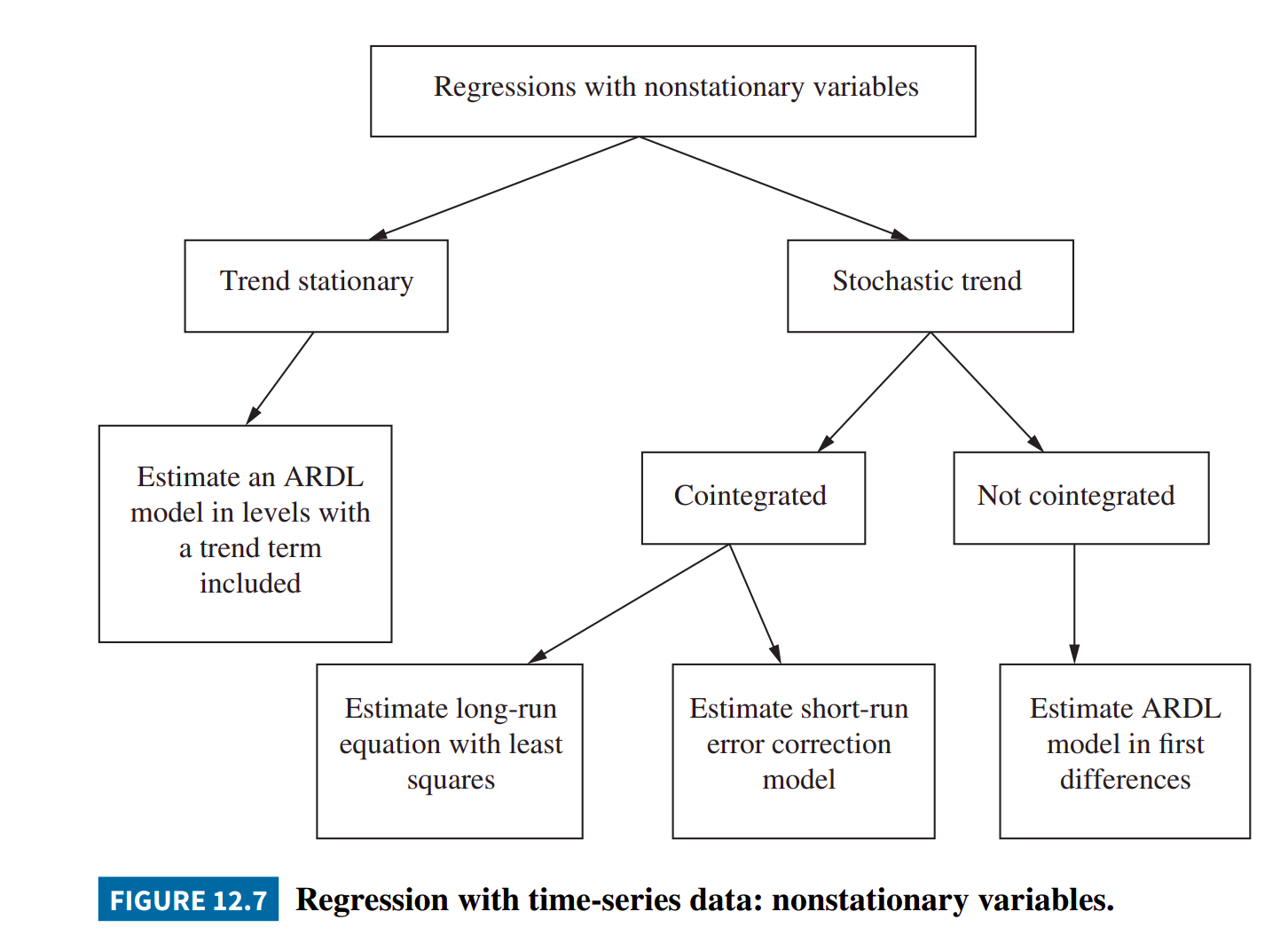
Regression with Time-Series Data: Nonstationary Variables
接下來Chp13 要講「VEC與VAR模型:總體計量經濟學的介紹」
VEC: Vector Error Correction
VAR: Vector Auto-regressive Models
VAR 適用於平穩變量的短期動態分析,而 VECM 進一步整合長期均衡機制,成為分析經濟變量協整關係的標準工具。兩者均廣泛應用於總體經濟預測、政策評估及金融市場關聯性研究。
老師回頭講Chpter 12 的p.584.
W15 Chp14- Time-varying volatility and ARCH models (II)
2025-05-28三 14:10-17:00 林師模教授
part 1: page 611, Chapter 13, Exercise 13.13, data file: equity,
Questions a, b, and c need to be explained b needs to do an indigenous test.
Part 2: choose a country, collect data for 40 years from the
database, after data collection, calculate the same as part 1, and
answer as in part 1.
variable: dividend, composite stock index, nominal dividend per
share.
就是第13章的某個Excersice
題目: 看p.610頁最下面 那個13.13 開始,一直到p.612開頭那a,b,c三個問題止(有兩個parts). 其實每個題目,都是在研讀某篇發表過的論文THE EQUITY PREMIUM A Puzzle*。
該論文提出了某種公式(就是找出了某種模型model),說是可以精確解釋某些現象。 這樣的宣稱,以及此model(數學公式)是否真能做出正確預測?就要經過許多學者、老師、學生反覆理解、不斷計算、檢查、挑毛病,最後才確立下來,最終被寫進教科書。
我有3個星期的時間,要搞清楚這論文到底說的是什麼?公式怎樣弄出來的,定義是什麼?怎樣運作又解釋了什麼?然後去回答a,b,c三個問題(part1)。
最後,還要找一個國家,利用他的40年紀錄資料,去驗證這個公式的精確性(part2)。
今天家裡有人來打掃,香香也陪著照顧、換藥,我正好躲在圖書館,看怎樣才能完成這個作業。打算是:
1st星期-至06-04三,讀懂論文說什麼和題目問什麼? |
Gimini-協助說明.pdf檔 |
2nd星期-至06-11三,回答abc(完成part 1),並開始找另一國家資料研究看看。
3rd星期-至06-18三,跑另一國家資料(完成part 2)。
W16 Chp14-Time-Varying Volatility and ARCH Models / Chp15- Panel data models (I)
2025-06-04三 14:10-17:00 林師模教授
老師的講義 Ch-13 | 教科書內容 Chapter-13 |
老師的講義 Ch-14 Time-Varying Volatility and ARCH Models | 教科書內容 Chapter-14 時變波動率和 ARCH 模型 |
老師的講義 Ch-15 Panel Data Model | 教科書內容 Chapter-15 面板資料模型 |
1.陳磊老師1 1 1计量经济学概述
2.1 1 2计量经济学的研究内容
3.1 2 1回归分析的基本概念
4.1 3 1回归方程的设定与估计
5.2 1 1一元回归模型的OLS估计
6.2 2 1多元回归模型的OLS估计
7.2 3 1OLS估计量的性质
8.2 4 1多元回归模型实例
9.2 5 1回归模型的拟合优度
10.3 1 1假设检验的概念對應教本第五章
11.3 1 2假设检验的判定准则
12.3 2 1置信区间法
13.3 2 2显著性检验法
14.3 3 1F检验的思路
15.3 3 2F检验的应用
16.3 3 3邹检验
17.3 4 1正态性检验
18.4 1 1遗漏变量与不相干变量對應教本第六、七章
19,4 1 2模型设定准则
20.4 2 1函数形式的选择
21.5 1 1多重共线性的定义對應教本第八章
22.5 1 2多重共线性的后果
23.5 2 1多重共线性的诊断
24.5 2 2多重共线性的补救
25.5 3 1多重共线性的案例
26.6 1 1序列相关性的概念与类型對應教本第九章
27.6 2 1序列相关性的后果和检验
28.6 3 1序列相关性的补救措施
29.7 1 1异方差性的概念和后果對應教本第十章
30.7 2 1异方差性的检验
31.7 3 1异方差性的补救措施
32.7 4 1异方差性的案例
33.8 1 1虚拟变量的含义對應教本第七和十六章的部份內容。
34.8 2 1虚拟变量的设置与引入Dummy veriable
35.8 3 1虚拟变量的应用
36.9 1 1虚拟应变量的概念對應教本第十三章的部份內容。
37.9 2 1线性概率模型
38.陳磊老師 9 3 1Logit模型和Probit模型
39.楊政老師 10 1 1预测及其步骤對應教本第十五章的部份內容。
40.10 2 1精度指标
41.10 3 1时间序列模型预测
42.11 1 1分布滞后模型的概念
43.11 1 2有限分布滞后模型的估计
44.11 1 3工具变量估计
45.11 2 1Granger因果关系 46.11 3 1平稳性
47.11 3 2单位根检验
48.11 4 1协整
49.11 4 2误差修正模型
50.12 1 1认识面板数据
51.12 2 1面板数据模型的设定
52.12 3 1面板数据模型的参数估计
53.12 4 1面板数据模型的设定检验
《計量經濟學》主要參考教材如下
1.高鐵梅
主編,《計量經濟分析方法與建模:EViews應用及實例(第3版)》,清華大學出版社,2016年
2.施圖德蒙德(A.H. Studenmund)著,杜江、李恒
譯,《應用計量經濟學(原書第6版或第7版)》,機械工業出版社,2011年或2017年
3.伍德里奇(J.M. Wooldridge)著,張成思
譯,《計量經濟學導論:現代觀點(第6版)》,中國人民大學出版社,2018年
4.古扎拉蒂(Damodar N. Gujarati)、波特 著,費劍平
譯,《計量經濟學基礎(第5版)》,中國人民大學出版社,2011年
5.肯尼迪(Peter Kennedy)著,陳彥斌、魏偉、宋雪
譯,《計量經濟學指南(第5版)》,中國人民大學出版社,2010年
6.斯托克(James H. Stock)、沃森 著,王立勇 譯,《計量經濟學(原書第3版
升級版)》,機械工業出版社,2021年
7.陳強
主編,《計量經濟學及Stata應用(第2版)》,高等教育出版社,2023年
W17 Chp15- Panel data models (II)
2025-06-11三 14:10-17:00 林師模教授
Reference:subject should study
W18 (Final Report)
須自習 Chp16- Qualitative and limited dependent variable models
2025-06-18三 14:10-17:00 林師模教授
Reference:subject should study
Backup Data 其他參考資料
Book | Data Miming | Data Science for Business |
URL | Kaggle | 彭明輝教授
1.演講Youtube: 期刊論文閱讀技巧
2.演講Youtube: 研究生的核心能力 ─ 從文獻回顧到批判與創新 │Future Faculty Talk
▼1 WHAT IS INFORMATION MANAGEMENT?
WHAT IS INFORMATION MANAGEMENT?
1.ANIMATION FOR PLATONWHAT IS INFORMATION MANAGEMENT? wearesynkro 2014。2. Information Management BasicsCommunity IT Innovators 2018。
3.(IM) Information Management JuanIT 2021。有一系列lecture
4.The 5 Components of an Information System COTC A.R.C. 2015。
▼2 自習課程-Ben Lambert、Bob、李宗璋老師
自習課程-Ben Lambert、Bob、李宗璋老師
牛津大學 Ben Lambert Econometrics | 筆記 | 李柏堅 CUSTcourses |【Mandarin國語】五分鐘計量經濟學(計量經濟學輔導)
第一集:什麼是OLS?
第二集:什麼是因果效應?
第三集:什麼是擬合值與殘差?
第四集:什麼是OLS擬合值與殘差的特點?
第五集:什麼是普通最小方差估計量的無偏特點? 第六集:什麼是高斯馬可夫定理?
第七集:什麼是“Ceteris Paribus”?
第八集:什麼是“零條件期望假定”和“零相關假定”?
第九集:什麼是SST,SSE,和SSR?
第十集:什麼是F統計量和F檢驗?
第十一集:什麼是R-squared和Adjusted R-squared?
第十二集:Stata回歸結果窗口有哪些統計量?
第十三集:什麼是遺留變量偏差?
第十四集:怎樣減緩遺留變量偏差?
第十五集:什麼是Frisch-Waugh-Lovell (FWL)定理?
第十六集:計量經濟模型與理論經濟模型的區別是什麼?
第十七集:如何描述對數變量和水平變量的系數估計值?
第十八集:經典線性模型的六個假設是什麼?
第十九集:什麼是內生解釋變量和外生解釋變量?Endogenous and exogenous explanatory variables
(phd19_Chapter 10 Endogenous Regressors and Moment-Based Estimation 隨機解釋變數撼動差估計)
第二十集:什麼是迴歸模型的矩陣表達形式?
第二十一集:如何推導矩陣形式的OLS估計量?什麼是投影矩陣和殘差生成矩陣?
第二十二集:如何推導OLS估計量(使用代數和矩陣)?
第二十三集:多元變量模型OLS估計量什麼時候跟部分模型OLS估計量相同?
第二十四集:什麼是矩陣的基礎概念和特點?
Economics in Real Life (Episode 5)
Episode 1 Income Inequality and Gini Coefficient
Episode 2 Game Theory and Prisoner’s Dilemma
Episode 3 Economic Development as Freedom
Episode 4 The Nature of Poverty
Episode 5 Tragedy of the Commons and the Overuse of Public Resources
Episode 6 Is A Bumper Harvest Always Good for Farmers?
Episode 7 Eviews 2 导入EXCEL文件
3.Eviews 3 绘制散点图
4.Eviews 4 估计回归方程
5.Eviews 5 主菜单简介
6.Eviews 6 series的操作
7.Eviews 7 group的操作
8.Eviews 8 equation的操作
9.Eviews 9 Jarque Bera test
10.Eviews 10 输出结果数值显示格式的设置
11.Eviews 11 多元回归
12.Eviews 12 受限最小二乘
13.Eviews 13 完全共线性
14.Eviews 14 多项式双对数倒数模型
15.Eviews 15 单个序列的绘图命令
16.Eviews 16 两个序列的绘图命令
17.Eviews 17 回归模型的命令
18.Eviews 18 虚拟变量的引入
19.Eviews 19 虚拟变量的交互项
20.Eviews 20 季节分析中的虚拟变量
21.Eviews 21 遗漏或多余变量的检验
22.Eviews 22 reset检验
23.eviews 23 多重共线性
24.Eviews 24 残差的图形诊断
25.Eviews 25 异方差检验
26.Eviews 26 加权最小二乘
27.Eviews 27 怀特异方差校正值
28.Eviews 28 自相关的图形诊断
29.Eviews 29 自相关LM检验
30.Eviews 30 广义差分变化
31.Eviews 31 Neway West校正值
32.如何使用Excel高级筛选工具?
EViews 14
▼3 自習課程-陳磊、楊政
自習課程-陳磊、楊政老師
1.陳磊老師1 1 1计量经济学概述
2.1 1 2计量经济学的研究内容
3.1 2 1回归分析的基本概念 對應教本第一章
4.1 3 1回归方程的设定与估计
5.2 1 1一元回归模型的OLS估计
6.2 2 1多元回归模型的OLS估计
7.2 3 1OLS估计量的性质
8.2 4 1多元回归模型实例
9.2 5 1回归模型的拟合优度
10.3 1 1假设检验的概念對應教本第五章
11.3 1 2假设检验的判定准则
12.3 2 1置信区间法
13.3 2 2显著性检验法
14.3 3 1F检验的思路
15.3 3 2F检验的应用
16.3 3 3邹检验
17.3 4 1正态性检验
18.4 1 1遗漏变量与不相干变量對應教本第六、七章
19,4 1 2模型设定准则
20.4 2 1函数形式的选择
21.5 1 1多重共线性的定义對應教本第八章
22.5 1 2多重共线性的后果
23.5 2 1多重共线性的诊断
24.5 2 2多重共线性的补救
25.5 3 1多重共线性的案例
26.6 1 1序列相关性的概念与类型對應教本第九章
27.6 2 1序列相关性的后果和检验
28.6 3 1序列相关性的补救措施
29.7 1 1异方差性的概念和后果對應教本第十章
30.7 2 1异方差性的检验
31.7 3 1异方差性的补救措施
32.7 4 1异方差性的案例
33.8 1 1虚拟变量的含义對應教本第七和十六章的部份內容。
34.8 2 1虚拟变量的设置与引入Dummy veriable
35.8 3 1虚拟变量的应用
36.9 1 1虚拟应变量的概念對應教本第十三章的部份內容。
37.9 2 1线性概率模型
38.陳磊老師 9 3 1Logit模型和Probit模型
39.楊政老師 10 1 1预测及其步骤對應教本第十五章的部份內容。
40.10 2 1精度指标
41.10 3 1时间序列模型预测
42.11 1 1分布滞后模型的概念
43.11 1 2有限分布滞后模型的估计
44.11 1 3工具变量估计
45.11 2 1Granger因果关系 46.11 3 1平稳性
47.11 3 2单位根检验
48.11 4 1协整
49.11 4 2误差修正模型
50.12 1 1认识面板数据
51.12 2 1面板数据模型的设定
52.12 3 1面板数据模型的参数估计
53.12 4 1面板数据模型的设定检验
《計量經濟學》主要參考教材如下
1.高鐵梅主編,《計量經濟分析方法與建模:EViews應用及實例(第3版)》,清華大學出版社,2016年
2.施圖德蒙德(A.H. Studenmund)著,杜江、李恒
譯,《應用計量經濟學(原書第6版或第7版)》,機械工業出版社,2011年或2017年
3.伍德里奇(J.M. Wooldridge)著,張成思
譯,《計量經濟學導論:現代觀點(第6版)》,中國人民大學出版社,2018年
4.古扎拉蒂(Damodar N. Gujarati)、波特 著,費劍平
譯,《計量經濟學基礎(第5版)》,中國人民大學出版社,2011年
5.肯尼迪(Peter Kennedy)著,陳彥斌、魏偉、宋雪
譯,《計量經濟學指南(第5版)》,中國人民大學出版社,2010年
6.斯托克(James H. Stock)、沃森 著,王立勇 譯,《計量經濟學(原書第3版
升級版)》,機械工業出版社,2021年
7.陳強
主編,《計量經濟學及Stata應用(第2版)》,高等教育出版社,2023年
▼9 折疊9
折疊2
- Lorem ipsum dolor sit amet.
- Lorem ipsum dolor sit amet.