W01 課程介紹
2025-09-10-Wednesday 14:10-17:00 林師模教授 shihmolin@gmail.com (助教Sophia張桂鳳Dr.)
| syllabus | phd16-QM(I) | Review of Statistics: Prof.'s: Basic Probability Concepts | 統計自習筆記 |
課本: Principles of Econometrics, 5th Edition | Formulas公式查表 | 課本的學習參考提示與答案 | 筆記: GoogleDoc
工具: p-value | t-critical value | wf1檔案定義 3rdEdition Data definition files (*.def)
作業: W03 Asig#1 | W07Asig#2 | W10Asig#3, [PDF] | W15Final Report | [PDF] |
考試: Exam | Midterm | Final |
同學:11304601劉珮彤Peyton, 11304625茉莉(India), (遇Romi同學-說統計很好的-Bisyri Effend想參加2026_LFHintern)
😊喜歡這門課,特地自動重修,這次希望可以盡可能找我們公司或自己感興趣的數據資料做研究。
本週在多倫多,請假!
W02 Review of Statistics
2025-09-17-Tuesday 14:00-17:00 林師模教授
Review of Statistics: Prof.'s: Basic Probability Concepts |
1.問? what's difference betweeen: standardizqtion and nomorlization
2.問? 為何需要standardization?
remove unit
confine the range, in -1<= sd <=1
esay to compare: for the unit has been removed
-注意frequently use公式: var(a+cX) = c^2var(X) 因為 a 是constant 沒有var (coefficient 係數)
-E[(X-EX) (Y-EY)] --> +or- will know the relationship of X and Y, that's call: covarance
雖然X-EX 或但是看不出來strength 這是因為 unit改變就會改變數字。如果想知道strength 強度,可以先做standarlilzation以除去unit。
所以可以用: Measure / SD
公式: Z = (Xi - EX )/S.D.(X)
-Cov(X,Y)=E[(X-EX) (Y-EY)] = {Sumation (X-EX) (Y-EY)} / n
看2,34 Correlation
is a pure number faling between -1 and 1
*注意 要在你的excel加上 增益集-分析工具箱-
這樣你按 資料時 右邊就會出現 「資料分析」這工具。
=自己用lireoffice和Googlesheet 試做個 x體重/y身高 資料表,然後叫他算出 correlation number 相關係數。
這工具還可有其他分析工具,但更複雜的要用Eviews之類軟體來做。
The coverse is not true. 這句話 Why?
Y=a+bX 時 cor = 1
但 如果是個圓的話 cor=0 但 X Y 應該是有關係 but why we got o relationship
因為只能測量 linear relationship 而如果你碰到non-linear relationship時,隨然 cor=0 但是X Y其實是有non-linear relationship的
-2.37
-2.38 記住 weighted sum of rendom variables: 的公式,很重要。常要用到。
問: 為何要sandardization?
答: 因為不可能弄無線多個distribution table, 如果把mean設為0 把sd設為1 那就只要一張table就好了!
probability ditribution table =
見 2.41 只要convaert 原來的Y變成a 做出 Standard normal
2.44 Chi-Square distribution
吸煙與肺癌的研究因為是從兩個獨立的群體(病例與對照)開始,並比較它們的吸煙習慣分布,所以它在統計學上屬於同質性檢驗的應用範疇。
2.46 F statistic distribution (F是偏左的 distribution 都是正的-因都平方, 右邊長尾)
i-learning_2.0
W03 ANOVA: Analysis of variance
2025-09-24-Tuesday 14:00-17:00 林師模教授
★ ■ ▲
wha is the steops of hypothesis
■ Hypothesis testing, ■ANOVA(Analysis of variance) 變異數分析;
ChatGPT說明 The
steps of hypothesis
例如: 100學生數學成績,內有分N M S 北中南三區學生
1.what question? is region -> effect of math score.
2.H0: μ1=μ2=μ3 (μN=μM=μS)
H1: μ1≠μ2≠μ3 either one ≠
3.★ select Test Statistic 檢定統計量 -找出critical value. (to know the
test statistic)
if the statistic not greater than critical value, fall in acceptance
area, means that you can not reject the H0.
- 如何找出test方法 經驗/自己推導-想辦法試驗/如果你不知道-you can develop
by yourself or even you can publish/ or use other people’s way, to know
how others usely do/.
- 多看別人的,多看文章,多看案例.
- ★ need to know what would be the porbability distribution (with your
test)
4. Collect Data and Calculate the Test Statistic
- need dicide alpha: significant value first (0.05 or 0.01,
0.10..)
consulting (F) talbe, then you can find out the coreponding critical
value.
★ Alpha value 的意義: TypeI error: Ho is true the probability of
rejecting the null only 5% (alpha)
你決定了alpha值,就是你決定可能犯了型1錯誤的機率,在alpha值之內。
- Find the Critical Value(s) or p-value
- Make a Decision
- State the Conclusion
■ANOVA(Analysis of variance)
if we have three or more normal distribution, and we would like to know
whether their means are the same or not?
比如剛剛那來自三個地區的100個學生,是否 H
可以求出一個total mean = μ
對任一個 (Yij-μ) = (Ynj-μj) + (μj-μ)
對所有n點想要總和,需要先square以免被相互抵銷
所以先 sauare (Yij-μ) 全部加總起來
SST (sum square total) = SSE (error sum of square 你自己母體的差) +
SSB (between group -sum square) 有時SSE 也叫做 SSW (Within group seim
square 的意思)
SST=SSE+SSB
如果各組差異大,那麼SSB會變大。 所以如果兩邊都除以SST 這樣就成了
1= (SSE/SST) + (SSB/SST) 假設 這是 1=0.3 + 0.7 那你怎麼知道
0.7有沒大過critical value?
如果各組差異大,那麼SSB會變大。 所以如果兩邊都除以SST 這樣就成了
1= (SSE/SST) + (SSB/SST) 假設 這是 1=0.3 + 0.7 那你怎麼知道
0.7有沒大過critical value?
問Gemini20250924
SST(sum square total), SSE (error sum of square), SSB (between group
-sum square)
設SST=SSE+SSB 所以 1= (SSE/SST) + (SSB/SST)
假如 SSE=0.3 而 SST=0.7 那要怎麼知道 0.7有沒大過critical value?
F Statistical calculation step:
F 統計量的計算公式通常是指變異數分析(ANOVA)中的 F = MSB / MSW,
其中MSB 是組間平均平方(Mean Square Between),
MSW 是組內平均平方(Mean Square Within),
F 值用於檢定多個母體平均數是否完全相同。
■ wiki F檢定
F 統計量的計算步驟
計算組間平方和(SSB):: 衡量不同組別之間的平均變異。
計算組內平方和(SSW)::
衡量每個組別內部數據點與該組平均數之間的變異。
計算自由度(df)::
組間自由度(dfB) = 組別數量- 1
組內自由度(dfW) = 總樣本數- 組別數量 (但老師在這個例題,用的是n-1
不是n-group number 因為是SST,但注意📌)
計算平均平方(MS):: 組間平均平方(MSB) = SSB / dfB
組內平均平方(MSW) = SSW / dfW
計算F 值:: F = MSB / MSW。
應用情境
變異數分析(ANOVA):: 這是F
統計量最常被使用的情境,用於比較三個或三個以上群體平均數的差異。
變異數比率檢定:: F 檢定也可以用於檢定兩個母體變異數是否相等。
如何理解F 值
F 值是組間變異與組內變異的比例。
較大的F
值表示組間的平均差異比組內的平均差異大,這暗示著群體平均數之間存在顯著差異。
📌注意: 正式用的是SSB /SSW 不是SST (SSW/m3 這個m3 就是df 就是 n-組別數量
)
F = (SSB/(J-a)) / (SSW/(n-J)) 老師說:根據經驗 n=100 J=3 時 Falpha .=.3 但如果J=5 可能小於3, 如果J=10 會更小。 不信去查F表。 F表最上面那行是group的df, 左邊直行是n的df。
老師要教。怎樣用excel去做F test data資料 –> data analysis資料分析 單因子變異數分析 –> by row 逐列: @回家用googlesheet 做看看。
ANOVA如果有 2 factor(如男女)但 sample數都一樣,叫做balanced table如果
sample數不一樣就是imbalanced table (如果每一類只有1個sample
data)叫做non-repetitions experiment非重複實驗 HomeWork:
老師出一個作業下週三以前sumit report, 題目是:
自己設計question自己收集data 做一個two factor ANOVA data
需要是repetition data.
這課會用到大量的統計、小部份的微積分推導,是好的學習機會。因此今年自動重修,準備重新進入頭痛的週三下午模式。
我們以前唸書先要買課本,有時還要買參考書。
現在的世界,很多課本、參考書都可以免費取得,如果你需要紙本的,再特別去買。
這是我們的課本,因為是免費的,所以也分享給各位。
Principles of Econometrics, 5th Edition
https://arm.ssuv.uz/frontend/web/books/643103c2ad0af.pdf
老師講得飛快,今天要講第二章
The Simple Linear Regression Model
稍不注意(比如沒有人提問、沒有討論)有時一週就把一章講完了(最多兩週),因此最好提早來先看例題,如果看不懂等一下就可以提出來問,拖慢腳步。
去年聽這個課,第1個小時好像懂,第2個小時好像不大懂,第3個小時一堆不懂。今年稍微好一點。
好在我有Gemini和ChatGPT還有Grok幫忙。一邊聽,一邊請教AI。
唉😢奇怪!今天老師不講OLS直接講■Hypothesis testing, ■ANOVA(Analysis of variance)。
Format for report: pdf file, less than 2 pages. 1.Descript your question. 2.Descript your variables and data. 3.ANOVA result. 4.Conclusions.
要回家拜託AI了 (這就是為什麼我要交錢給ChatGPT和Gemini)
我跟Gemini討論用Eviews8.1做ANOVA的過程我跟ChatGPT討論用python做ANOVA的過程
W04 Chp02-The Simple Linear Regression Model
2025-10-01-Tuesday 14:00-17:00 林師模教授
- Mastering Econometrics with Joshua Angrist
- 有例題可作 簡單線性迴歸分析
- University of West Georgia Linear_regression_Notes
2.高點研究所 研究所碩士班歷屆考古題 #statistics
3.NotebookLM 肥料效益差異的F檢定與事後分析
ChatGPT20250924
關於迴歸模型Regression
model:請解釋估計量estimator和估計值estimate之間的區別,以及為什麼最小平方法估計量least
squares estimators是隨機變量,而最小平方法估計值不是。
經典線性迴歸假設
1.線性模型:
2.誤差項的期望值為 E[Ui]=0
3.誤差項變異數齊一 var(Ui)=σ^2
4.誤差項不相關 Cov(Ui,Uj)=0, i≠j
5.解釋變數不完全共線
Classical Linear Regression Assumptions
1. Linear Model:
2. The expected value of the error term is E[Ui] = 0
3. The variance of the error terms is uniform (var(Ui) = σ^2)
4. The error terms are uncorrelated (Cov(Ui,Uj) = 0, i ≠ j)
5. The explanatory variables are not completely collinear.
Youtube Introduction To
Ordinary Least Squares With Examples
「珂学原理」No.94什么是最小二乘估计?它解决什么问题?
- If you are rusty or uncertain about probability concepts, see the
Probability Primer and Appendix B at the end of this book for a
comprehensive review.
The Simple Linear Regression Model
Why?
simple: one dependent variable has only one independent
variable.
Linear: relationship: the equation show as a line.
regression: (regress vs. progress 進步) use the already data to
look back the relationship. observe the relationship of data. useing the
data in the past to generate a line to look back the relationship.
model: from emperical phenomeno to abstract the idea, make
specification of a relationship.
例如: y: expenditure x:income
y=f(x) base on economic model
we might be able to build up a true function of the model by collecting
empirical data of observation.
so we may say: y=β1 + β2 x (this is a emperical model)
true value like (xi, yi) may differenct from (xhat, yhat) which is on
the regression line. so we have turn the model to: yi= β1 + β2 xi + ei
(this is a econometric model) we need to use true data to estimate the
β1,β2,ei parameters
yi= β1 + β2 xi + ei
y: dependent, explained被解釋, regressant, response variable
x: independet, explanatory, regressor variable
ei: erro term, residule(after we estimate model),
β1 and β2: regression coefficient, parameter
β1: intercept, constant
β2: slope (=dyi/dxi = deribative 導數 =when detax change one unit, deaty
change ratio = marginal effect 邊際效應 = 當你有一個exiting situation
增加一個unit叫做 marginal unit)
這個existing situation很重要,因為可能是個critical point,
越過這個existing situation狀況可能改變,但marginal
effect不隨狀況改變。
所以在這裡的modle 這個β1是個constant 和β2 是個(線性的)slope
都不會變,是個marginal effect。
注意:如果是個曲線 那麼slope 會改變,就不能算是marginal effect。
β2=dy/dx 是個marginal effect
econometric model = regression model
for every econometric model we always needs an Assumptions.
there are many Assumptions, we will look at it one by one.
今日的Quick Review:
example: 2 variable: Income=x, Expenditure=y
more income will expend more money, so there is a linear relationship.
so we can set up a model:
yi= β1 + β2 xi
the distance from xi to the line we call it erro term (ei) thus come out
the econometic model:
yi= β1 + β2 xi + ei
想找出β1,β2就要根據assumption 的定義
1.linear relationship
2.E(ei | xi) =0
3.Cov(xi,ei | xi) =0
4.Cov(ei,ej | xi) =0
5.xi is nonstotastic
6.ei~ N(0,σ^2)
find out the best line: estimation (estimate a value for model ):
least square idea is let the total distance from data point to the line
should be smallest: the sumation of all erro term shoud be minimized. in
case of the summation became 0, we should square it then do the
summation.
after you summation of square will became a quadratic line, then we
should do firest derivative to find out the tangent line.
得出公式!!!!!!! get regression model.
老師展示example: 用Eviews:
food.wfi
先選ubcome再ctrl+foodexp open by group
Quick>estimate equation> [food_exp c income ] method: LS-least
squares
OK>就可得到estimate result
W05 Chp02-The Simple Linear Regression Model
2025-10-08-Tuesday 14:00-17:00 林師模教授
講義: Ch-02 Simple Linear Regression Model
講義: Ch-03 Interval Estimation and Hypothesis Testing
This is a regression model and also an econometric model.
we have no population so throug sample we get we estimate parameter β2.
(2) yi = b1 + b2 xi + ei^ (sample: estimator model)
b1, b2 are estimators of β1, β2
we call ei^ as resedule.
(3) yi^= b1 + b2 xi (call sample regression line)
acording by (2)(3) we can estimate: ei^ = yi - ( b1 + b2 xi) = yi - yi^
(yi^ is fitted value of yi, also called pedictied value)
OLS: Ordinary Least Square:
b1 = ybar - b2 xbar
b2 = cov(x,y) / var(x)
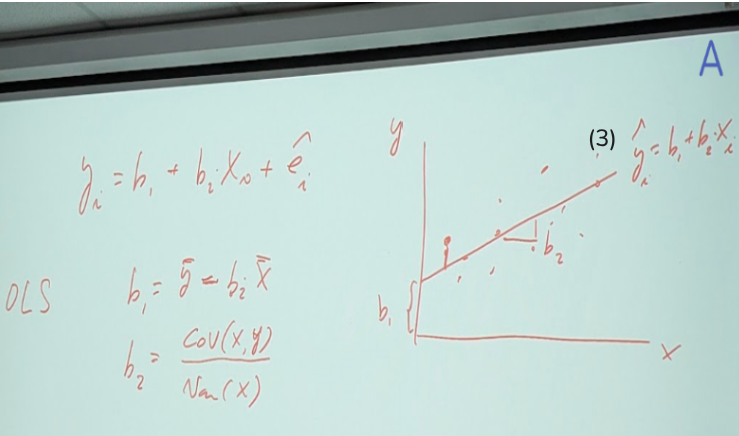
圖: a (下面還有公式)
複習Assumption of Least squaqre (注意-2,3-更正上週說法)
1.linear relationship
2.E(ei | xi) =0 has two implications(兩層意義): E(ei)=0 and
Cov(xi,ei|xi)=0
(見📌講義p.9 2.1 )
3.var(ei|xi) =σ^2
4.Cov(ei,ej | xi) =0
5.xi is nonstochastic (非隨機的)
6.ei~ N(0,σ^2) -> ( σs2= Σ(ei-ebar)^2 / n = Σ(ei)^2 /n )
σhat2= Σ(ei^ - e^bar )^2 / (n-1) = Σ(ei^) ^2 /(n-1)
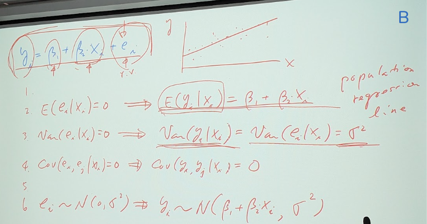
圖: B相片
2.E(ei | xi) =0 so-> and E(yi | xi) = β1 + β2 xi (=population regression line)
3.var(ei|xi)=0 so-> var(yi|xi)= var(ei|xi) =σ^2
4.Cov(ei,ej | xi) =0 so-> Cov(yi,yj | xi) =0
5.
6.ei~ N(0,σ^2) so-> yi~ N(β1+β2xi,σ^2)
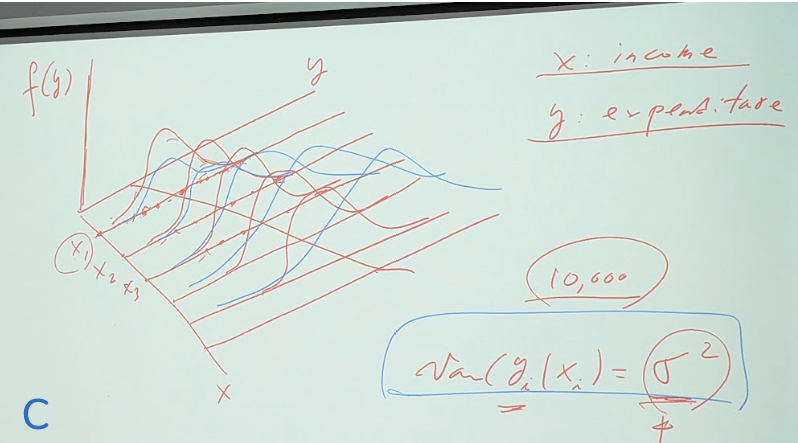
圖: c 相片 立體圖用 income/expenditure為例 (下面還有公式)
不同的x(比如xi=$1,000元)會有很多y點(expenditure)的分佈
每條x上的y 都會是normal distribution
📌講義p.8 2.2.1 All
pairs drawn from the same population are assumed to follow the same
joint pdf and are identically distributed i.i.d
(理論上: 每條y的distribution 變異數variance都一樣所以樣子都一樣)
理論如此,但實務上不會那麼剛好,所以可能像藍色線那樣分佈。
以上是Quick Review for Basic Concept
現在看講義快速過一次, 有10節 但有些節會跳過去(可回家自己慢慢看)
📌講義p.4 2.1 The
pdf f(y) describes how expenditures are distributed over the population
since Households with an income of $1000 per week would have various
food expenditure per person for a variety of reasons.
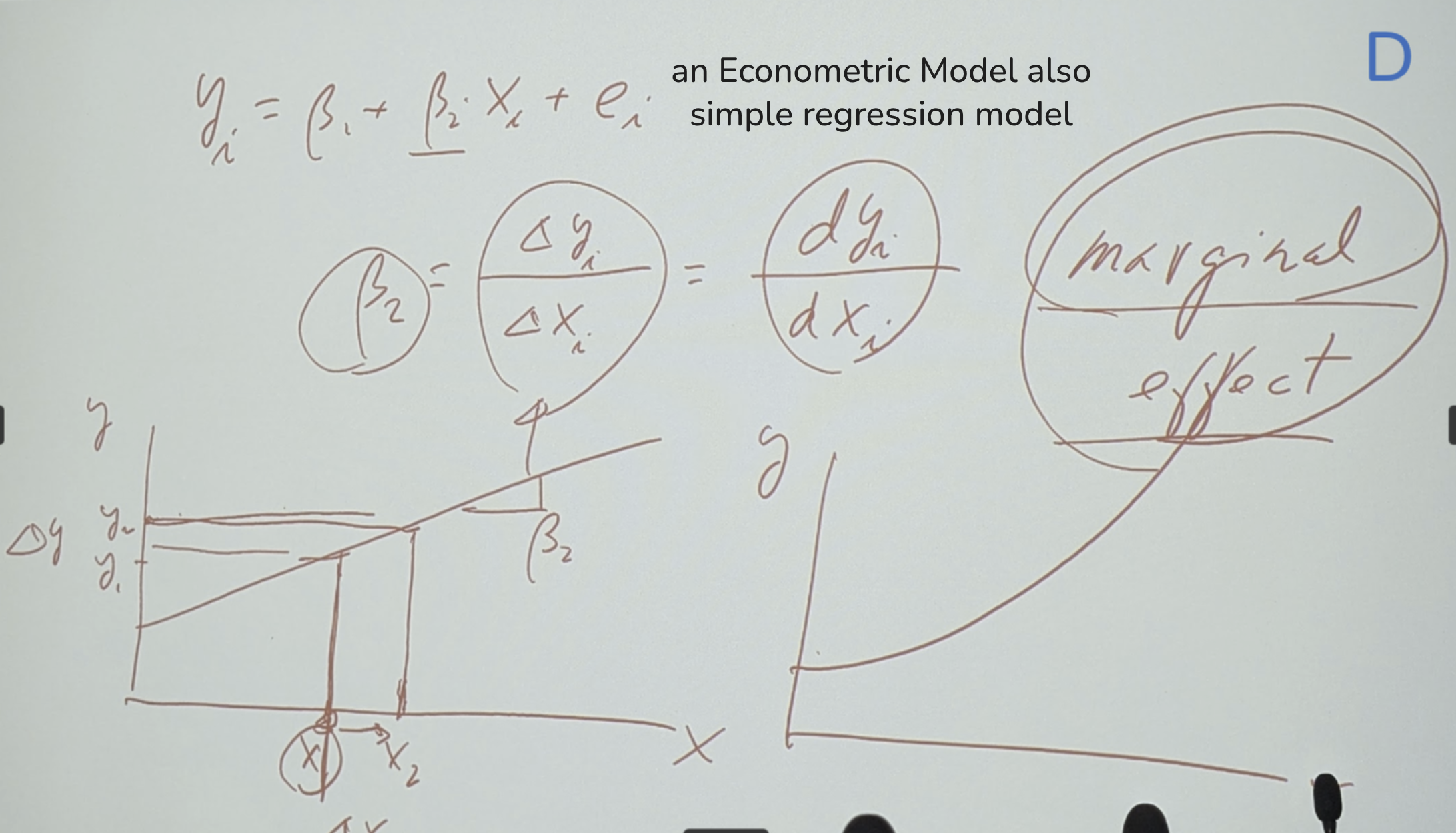
2.2 exogeneity 外生性; 複習為什麼economic model上叫做 marginal effect
(看圖d β2=dyi/dxi) will depend on your current situation, always the
same. 2.2.4 𝑣𝑎𝑟 𝑒𝑖 𝑥𝑖 = 𝜎2 This is the homoskedasticity (homo=same;
skedasticity=variance)
📌講義p.18 2.2.9
Summarizing the Assumptions 接下來p.19舉例:
想想我們怎樣找出這個yi^ 看p.21 (2.5) (2.6) 如何去fitted
regression line
which is: the Best Linear Unbiased Estimators. We call this is BLUE estimaors是一個formular, 就是說: 這個formular一旦用OLS方法可以找出b1,b2 我們就稱這個formular是BLUE。
至於為什麼?你可以去看教科書的附錄,那裡有BLUE的公式推導證明。
📘課本 p.375 8.4.1 Transforming the Model: Proportional Heteroskedasticity
看講義p.23有b1,b2的公式
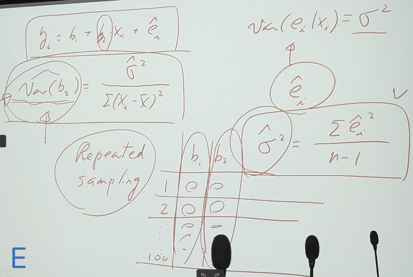
var(b2) = σhats2 / Sumation(xi-xbar)^2 and σhats2 = ehati s2 /n-1
請參考講義p.29- 2.4.3 Sampling Variation
奇怪,b2不是只有一個數字嗎,怎會有var(b2)? 這是因為 因為有Repeated
sampling的關係 見相片F 有表格 b1 b2 1,2,3….100
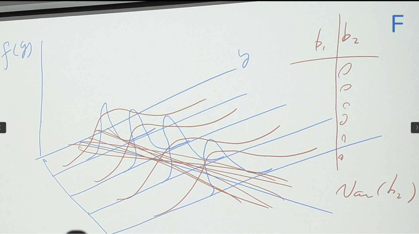
會何需要用這想法?你就要回去看立體圖 相片(圖: c) 因為x1…xi 每個x會有很多不同的yi 這樣很多linear line會有不同的var(b2) 看見相片f
(跟c很像的立體圖 但有var(b2)公式) 當你作了很多Repeated sampling 後, var(b2)可看出是寬或窄 你的母體怎樣 sampling就會長怎樣 你只要看Repeated
sampling的var(b2)就可看出分佈是寬或窄
b2最重要 他就是marginal effect 請記住公式(2.15)
Exercise food.wf1 重跑Eviews 展示: income +ctl expenditure > open as group > view -ploat sactter + fited line= regression line Quick: estimate equation : expenditure c income > method default to LS -確定 > 解讀result: C INCOME 你可以看到b2 就是income的 SD 他的square就是 var(b2)
如果你想產生y^ -> 去做Forcast (他增加一個food_expf 新的變數 focast的意思) income +ctl expenditure +cal food_expf> open as group > view -ploat sactter + fited line= regression line 就可以看到focast 的線條
income +ctl resid > open as group > view -ploat sactter 可看到residule 分佈
Residule不用管大或小,但在意是不是constant?
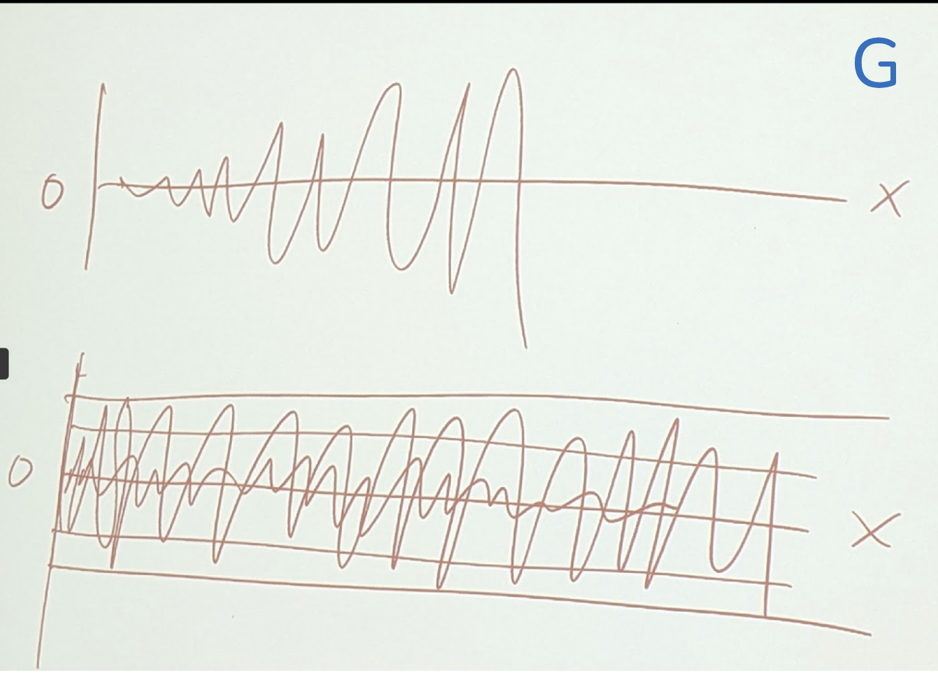
看圖G: 所謂constant就是 在一定範圍內震盪(變化),而不是越來越大或越變越小。
舉另外一例 📌講義p.47 2.2.9 Figure 2.14 A Fitted Quadratic Relationship
因為原先x,y的關係是Quadratic Relationship而非Linear Relationship,怎麼辦呢?有兩種方法可以嘗試: 1.是把independent variable SQFT再square一次 設法把曲線變為線性關係
2.另一方法是處理dependent variable y,把y做Logarithmization,即 log y也可以
但兩種方法需要比較,看那個線型比較好? (以能和最多iPair發生關係的最好)
現在用EXAMPLE 2.6 Baton Rouge House Data 來做練習 (使用資料檔br.wf1)
- sqft + ctl price > open as group > view -graph -sactter >看起來不像learning Eviews有兩種方法可run qudratic or log equation:
- price c sqft^2 > result > forcast pricef (fitted value) 會出現變數 pricef 這是第一個model
- sqft + ctl price + ctl pricef > open as group > view -graph-sactter
- log(price) c sqft > result > forcast pricef2 (fitted value) 會出現變數 pricef2 這是第2個model
- sqft + ctl price + ctl pricef2 > open as group > view -graph-sactter -ok
將兩個圖疊起來做比較,看誰比較線性!
- sqft + ctl price + ctl pricef2 + ctl pricef > open as group > view -graph -sactter -ok
那一個比較好?請看講義p.52的討論: 2.8.5 Choosing a Functional Form
(在這個case是 (2)比較好,因為他可以掌握最多的資料)
作業:📘課本
p.93這個練習
2.11.2 Computer Exercises
The capital asset pricing model (CAPM) is an important model in the field of finance. It explains variations in the rate of return on a security as a function of the rate of return on a portfolio consisting of all publicly traded stocks, which is called the market portfolio. Generally, the rate of return on any investment is measured relative to its opportunity cost, which is the return on a risk-free asset. The resulting difference is called the risk premium, since it is the reward or punishment for making a risky investment. The CAPM says that the risk premium on security j is proportional to the risk premium on the market portfolio. That is:
rj - rf = βj ( rm - rf )
rj − r = αj + βj ( rm − r ) + ej
b. In the data file capm5 are data on the monthly returns of six firms (GE, IBM, Ford, Microsoft, Disney, and Exxon-Mobil), the rate of return on the market portfolio (MKT), and the rate of return on the risk-free asset (RISKFREE). The 180 observations cover January 1998 to December 2012. Estimate the CAPM model for each firm, and comment on their estimated beta values. Which firm appears most aggressive? Which firm appears most defensive?
c. Finance theory says that the intercept parameter αj should be zero. Does this seem correct given your estimates? For the Microsoft stock, plot the fitted regression line along with the data scatter.
d. Estimate the model for each firm under the assumption that αj = 0. Do the estimates of the beta values change much?
下週要開始第3章講 Interval Estimation and Hypothesis Testing
W06 Chp03 Interval Estimation and Hypothesis Testing
2025-10-15-Tuesday 14:00-17:00 林師模教授
課本: Principles of Econometrics, 5th Edition | Chp03 第112頁開始。
講義: Ch-03 Interval Estimation and Hypothesis Testing | Youtube Descriptive Statistics vs Inferential Statistics |
溫故知新: Quick Review of Chp.02
最重要的3個公式
(1)yi =β1 + β2 xi + ei (econometric,regression model; population regression line)
(2)yi =b1 + b2 xi + ei^ (sample estimator model; b1,b2 are estimators of β1, β2; call ei^ as residule)
(3)yi^=b1 + b2 xi (call sample regression line)
以food.wf1為例,用Eviews跑資料:
Estimation Command: LS FOOD_EXP C INCOME
Estimation Equation: FOOD_EXP = C(1) + C(2)INCOME
Substituted Coefficients: 就得到結果如下,以及下表
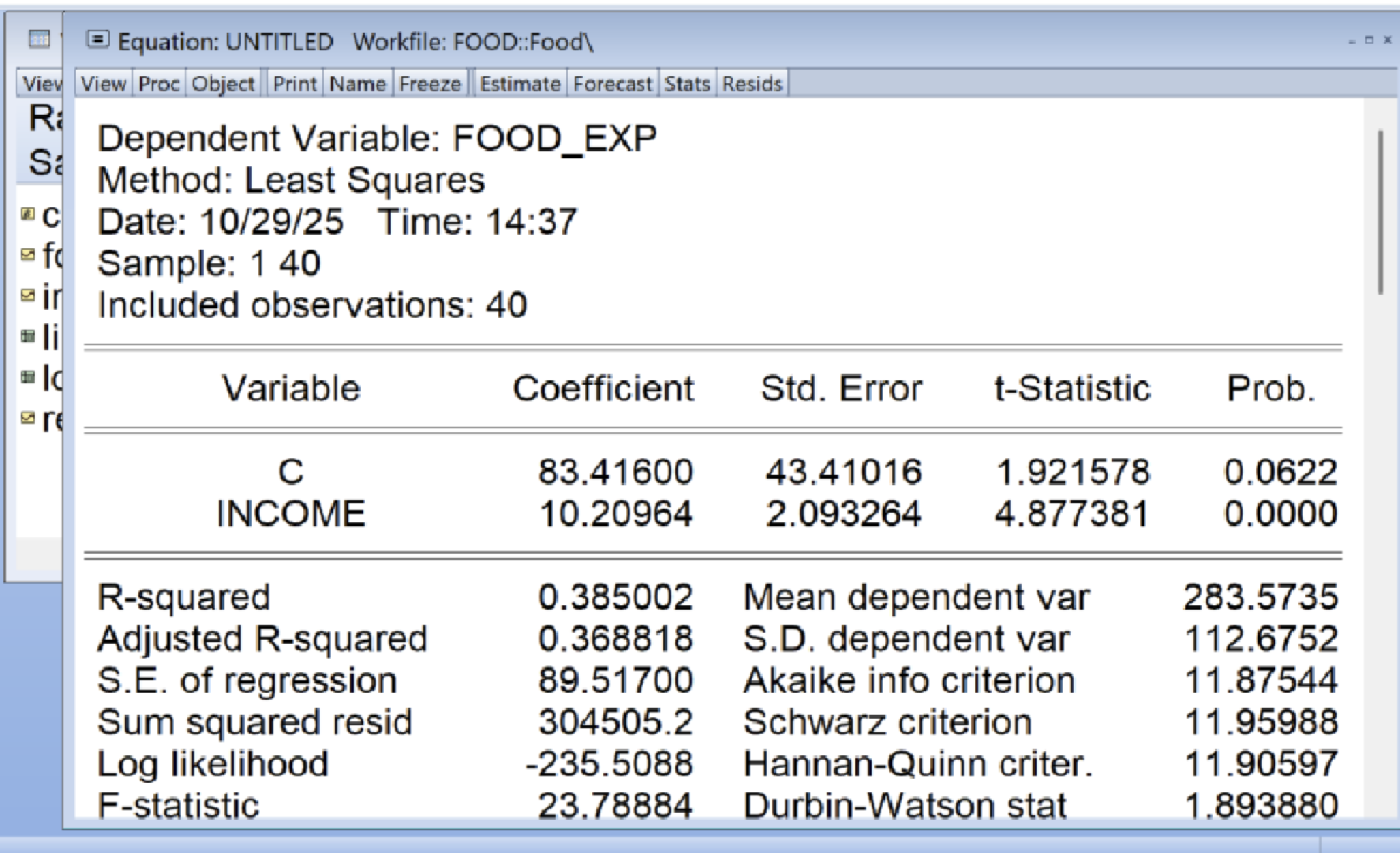
FOOD_EXP = 83.4160020208 + 10.2096429681INCOME
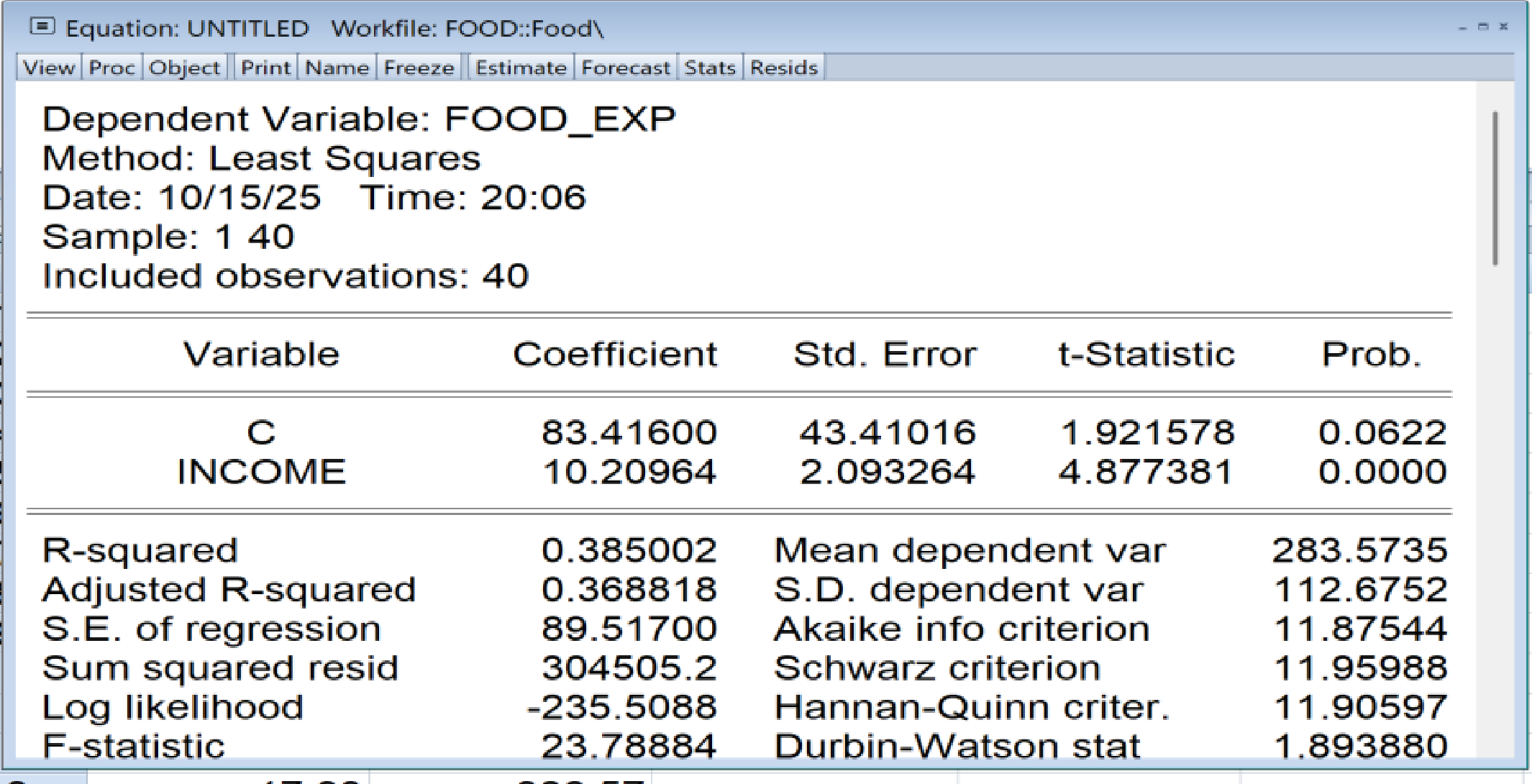
(表1)
清楚知道:
C (就是b1) 係數等於 83.41600 標準差Std.Error是 43.41016
INCOME (就是b2) 係數等於 10.20964 標準差Std.Error是 2.093264
而且(表1)表格中說:
S.E. of regression = 89.51700 (把這個squared就是 σ^2)
Sum squared resid= 304505.2
Mean dependent var =283.5735 (這就是 y bar)
S.D. dependent var =112.6752
現在我們要來研究 var(β2):請看
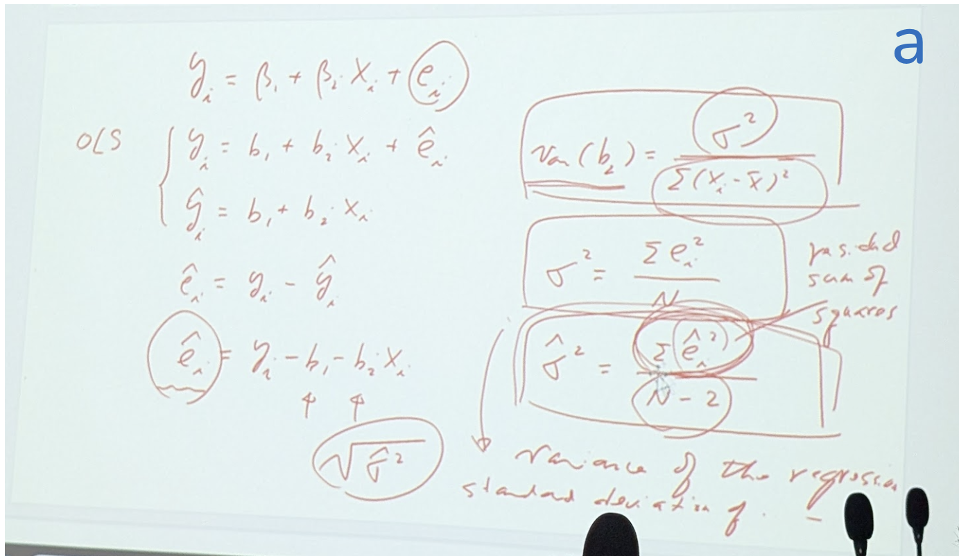
(圖a)
因為 var(β2)= σ2 /
Σ(xi-xibar)2
那首先就要先弄清楚σ2
和Σ(xi-xibar)2 的值。
1.σ2: Sum squared residule的公式是 σ2 =
Σ ei2 / N 但因沒有population只有sample,
所以改用 σ^2 = Σ ei^2 / N-2
(少掉b1,b2兩個)
因為Eviews已算出 Sum squared residule =304505.2 這就是Σ
ei^2,
而將這個Σ ei^2開根號(再除以38)就是S.E. of
regression = 89.51700 這就是σ^2
(反之: (89.51700)2 * 38= 304505.144982 =Sum squared
residule)
因ei^ = yi -b1 -b2 xi (失去b1,b2兩個的df)
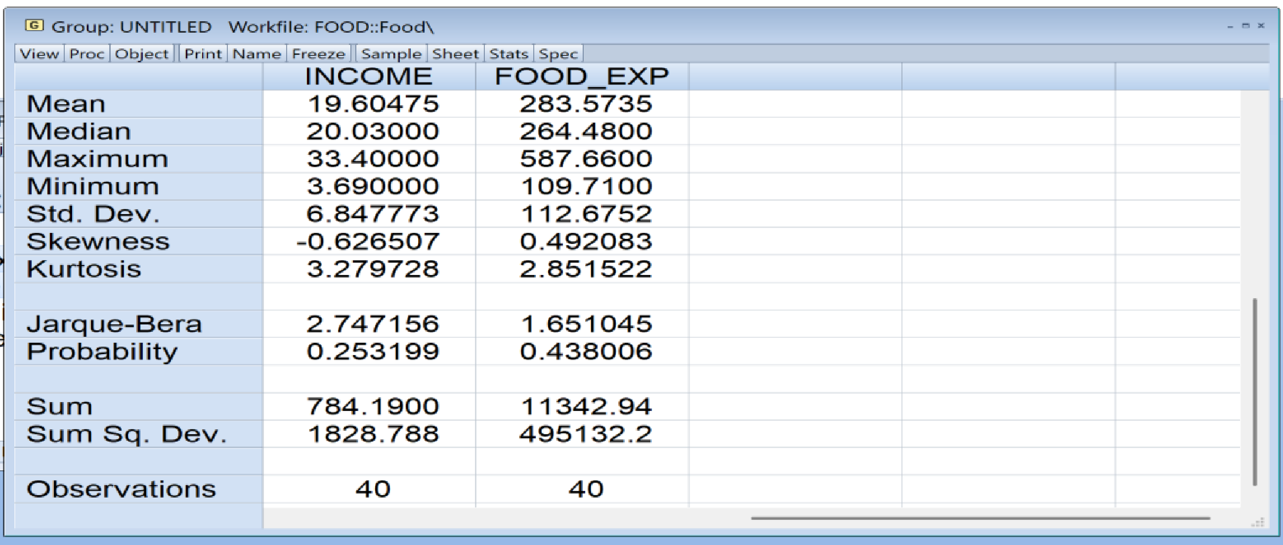
(表2)
2. Σ(xi-xibar)2:
因為 var(x) = Σ(xi-xibar)2 / N-1 在Eviews選變數[income+Ctl
food_expd]->Open with group->view->Discriptive Stats->Common
Sample就會出現 (表2)可看到:
Std. Dev. of INCOME 也就是 x 的 Std. Dev.= 6.847773
Std. Dev. of FOOD_EXP 也就是 y 的 Std. Dev.= 112.6752
公式 var(x) = Σ(xi - xi bar)2 / N-1
所以Σ(xi - xi bar)2 = (Std. Dev of x)2 *
(N-1) = 6.8477736.84777339 =1828.788
現在我們會算也會看這些關係了,可以知道各個 value of regression。
now we interested in var(b2) let’s move on Chp.03
開始講第3章:
Interval Estimation:
b1 and b2 we call estimators, when get value of b1 and b2 so call
estimate.
they are called “point estimate” 點估計; empericaly some time we might
not just interested just one point, instead, interested in a range. an
interval.
那麼range怎樣找出來呢?
idea is “how can we get range” how to establish?
(1) yi = β1 + β2 xii +
ei (call population regression line)
(2) yi = b1 + b2 xi +
ei^ (sample: estimator model)
用Z公式來standardize b2
Z=b2 -β2 /Se(b2) = (StdE(b2)
請參考前面的 var(b2) 公式) StdE(b2)=se=standard error
請照著講義p.4-5 的說明展開程式,就可找出做interval的正確方法。
先standardize b2在決定confidence value-找出z value
再用公式算出interval
slightly different from Z to t, because we do not know σ only know
σ^
注意: 因為沒辦法用 sigama square 需要換成 sigama hat square 所以Z
distribution 要換成 t distribution
注意p.7 的 (3.2)公式 的 根號中的σ square 應該改為 σ hate square
才對。
注意t table查表 時須注意正確的degree of freedom.
(課本863頁TABLE D.2 Percentiles of the t-distribution查95%-1.685/df38
如果到了∞ 也是1.96和Z一樣)
- p.862-Z表TABLE D.1是查: Cumulative Probabilities for the Standard
Normal Distribution (z) = P(Z ≤ z)
注意: p.10 tc 也寫錯了 應該是 bk 才對!!
回課本p.116 去看EXAMPLE 3.1 Interval Estimate for Food Expenditure
Data
老師用food.wf1跑一次Eviews來解釋interval作法:
- food_exp c food ->Std. Error
你可以用公式自己算,也可以按按Eviews就可以輕鬆算出
- view-> coeffice diagnostics-confidence interval-chose a
confidence-或3個都要或改都可以->OK就算出來了
想想這三種confidence的interval的意義。
- 看看TABLE 3.1, 3.2 分幾次 每次只取10個sample去跑 會怎樣?
A:用「Quick」: EViews>Quick>Estimate Equation
輸入equation: xom_rf c mkt_rf
備註:
xom_rf=(rj - rf) 是因變數。
c 是常數項 (αj)
mkt_rf=(rm - rf) 是自變數。
B:也可用: 工作檔視窗點選xom_rf(再Ctrl 依序) +c (若沒選也可以在下一步驟中手動添加) +mkt_rf >右鍵Open>as Equation.
彈出Equation Specification視窗,並預填公式,若需要時此時可補填入 c >OK。
得出結果後: View>Coefficient Diagnostics>Cinfidence Intervals...>OK
就會得到 0.9 0.95 0.99 三個Cinfidence Intervals的low和hight beta value.
0.315325 < MKT_RF < 0.597717
回去要詳看一次: 課本的學習參考提示與答案
接下來p.118要講3.2:
Hypothesis Testing:
- yi = β1 + β2 xi +
ei (call population regression line)
- yi = b1 + b2 xi +
ei^ (sample: estimator model)
只要有sample總是可以得到b1 b2 (比如food的結果如下)
yi = 83.41 + 10.2 xi + ei^ 但實際上不是那麼可靠!
但如果 β2=0 表示 x沒有 effect對於y
那麼10.2 一直到趨近於0 之間,到那一個點(critical point)這個effect會變得very weak?!
這就需要做test 看看 β2=0 是否成立! 看看在這個(critical point)時 是不是significant 說他們是有顯著的關系。
如果significant 就是
H0: β1=0
H1: β1≠0
H0: β2=0
H1: β2≠0
t = b2-β2 /Se(b2) ~ tα/2, N-2
α=0.05 so α/2=0.025
4.8已進入 rejection area, which is means β2≠0, it is
significantly different from 0.
because t vale is greter than critical value (超出了α 的critical
point)
這是針對單一回歸係數的檢定!
這在3.2.2有更詳細的解釋 需要去看
還有3.3.1講的是單尾的假設檢定
下週W07-從p.123的3.4 Examples of Hypothesis Tests開始講
下課了,真好。
W07 Ch-03 Interval Estimation and Hypothesis Testing
2025-10-22-Tuesday 14:00-17:00 林師模教授
課本: Principles of Econometrics, 5th Edition | Chp03 第123頁開始。
講義: Ch-03 Interval Estimation and Hypothesis Testing
期中報告
Interval estimation is a procedure for creating ranges of values, sometimes called confidence intervals, in which the unknown parameters are likely to be located.
Hypothesis tests are procedures for comparing conjectures that we might have about the regression parameters to the parameter estimates we have obtained from a sample of data.
depend very heavily on assumption SR6
SR6:
ei~ N(0,σ2) -> ( σ2= Σ(ei-ebar)2 / n = Σ(ei)2 /n )
σ^2= Σ(ei^ - e^bar )2 / (n-1) = Σ(ei^)2 /(n-1)
p.114 interval formular derivation: The statistical argument of how we go from (3.1) to (3.2) is in Appendix 3A.
p.115 [3.1.2] Obtaining Interval Estimates
(3.4) P(−tc ≤ t ≤ tc) = 1 − α
P[−t(0.975, N−2) ≤ t ≤ t(0.975, N−2)] = 0.95
(3.5) P[bk +- tcse(bk)] = 1 - α
W07-從p.123的3.4 Examples of Hypothesis Tests開始講
1. Determine the null and alternative hypotheses.確定零假設和備擇假設。
2. Specify the test statistic and its distribution if the null hypothesis is true.若虛無假設成立,則指定檢定統計量及其分佈。
3. Select α and determine the rejection region.選擇α並確定拒絕域。
4. Calculate the sample value of the test statistic.計算檢定統計量的樣本值。
5. State your conclusion.陳述你的結論。
(老師的講義)
1. A null hypothesis 𝐻0
2. An alternative hypothesis 𝐻1
3. A test statistic
4. A rejection region
5. A conclusion
When testing the null hypothesis that a parameter is zero, we are asking if the estimate b2 is significantly different from zero, and the test is called a test of significance.
統計檢定程序無法證明零假設的真實性。當我們無法拒絕零假設時,假設檢定所能確定的只是資料樣本中的資訊與零假設相符。
“If a value of the test statistic is obtained that falls in a region
of low probability, then it is unlikely that the test statistic has the
assumed distribution, and thus, it is unlikely that the null hypothesis
is true.”
“如果獲得的檢定統計量的值落在低機率區域,則檢定統計量不太可能具有假定的分佈,因此,零假設不太可能為真。”
” If the alternative hypothesis is true, then values of the test
statistic will tend to be unusually large or unusually small. The terms
“large” and “small” are determined by choosing a probability α, called
the level of significance of the test, which provides a meaning for “an
unlikely event.” The level of significance of the test α is usually
chosen to be 0.01, 0.05, or 0.10.
” 如果備擇假設成立,則檢定統計量的值往往會異常大或異常小。
「大」和「小」這兩個術語是透過選擇一個機率α來確定的,該機率被稱為檢定的顯著性水平,它為「不太可能發生的事件」提供了含義。檢定的顯著水準α通常選擇為0.01、0.05或0.10。”
Type I error If we reject the null hypothesis when it is
true, then we commit what is called a Type I error
- we can specify the amount of Type I error we will tolerate by setting
the level of significance α
Type II error If we do not reject a null hypothesis that is
false, then we have committed a Type II error
- we cannot control or calculate the probability of this type of
error
After we have estimator, somtimes we needs to know whethere there is
meaning of the parameters: coefficent-b2 (or b1)
whethere we can use the estimat LINE to represent the estimation?
we needs to TEST
set H0: β2=0
H1: β2 != 0
where the normaly distribution of be β2 : we use t-test to see if the average is 0 or not?
p.123 run Eviews [EXAMPLE 3.2 Right-Tail Test of Significance] 用 food.wf1
equation: food_exp c income
(表1)
但如何嚴謹的推斷、證實這個假設呢(即b2>0)?我們可以做一個
Null Hypothesis(虛無假設)H0:β2 = 0。
再設一個對立假設H1:β2 > 0。
如果我們拒絕了零假設(虛無假設)H0,我們可以直接得出結論:β2 為正,並且只有很小的機率(α)我們犯了錯誤。 此假設檢驗的步驟如下:
1.設定H0,兩個假設H1。
2.指定檢定統計量及其分佈。(是抽樣,所以用t分佈。
而因為設若null hypothesis H0:βk=c為真。那麼這公式就推導為:
(3.7) 統計量 t=(bk-C) / se(bk) ~t(N-2)
而目前根據H0的設定,c=0 因此,(💡t value)統計量 t= bk / se(bk) ~t(N-2)
4.經Eviews計算我們得到b2=10.21和se(b2)=2.09所以, t=b2 / se(b2) = 10.21/2.09 =4.88
5.由於 t = 4.88 > 1.686,我們拒絕虛無假設 β2 = 0,並接受備擇假設 β2 > 0。
結論:
We reject the hypothesis that there is no relationship between income and food expenditure and conclude that there is a statistically significant positive relationship between household income and food expenditure.

(圖a)
關於這P-value: 注意相片b "P-value"就是藍色部份 (可以拿p vs. α) 比如這裡 p=0.03 比 α(alfa) 0.05還要小
所以已經進入rejection region了,所以要reject H0.
所你也可以看t-Statistic value 也可以看 P-value (Prob)這會快多了,你不用去查t-table比對tc
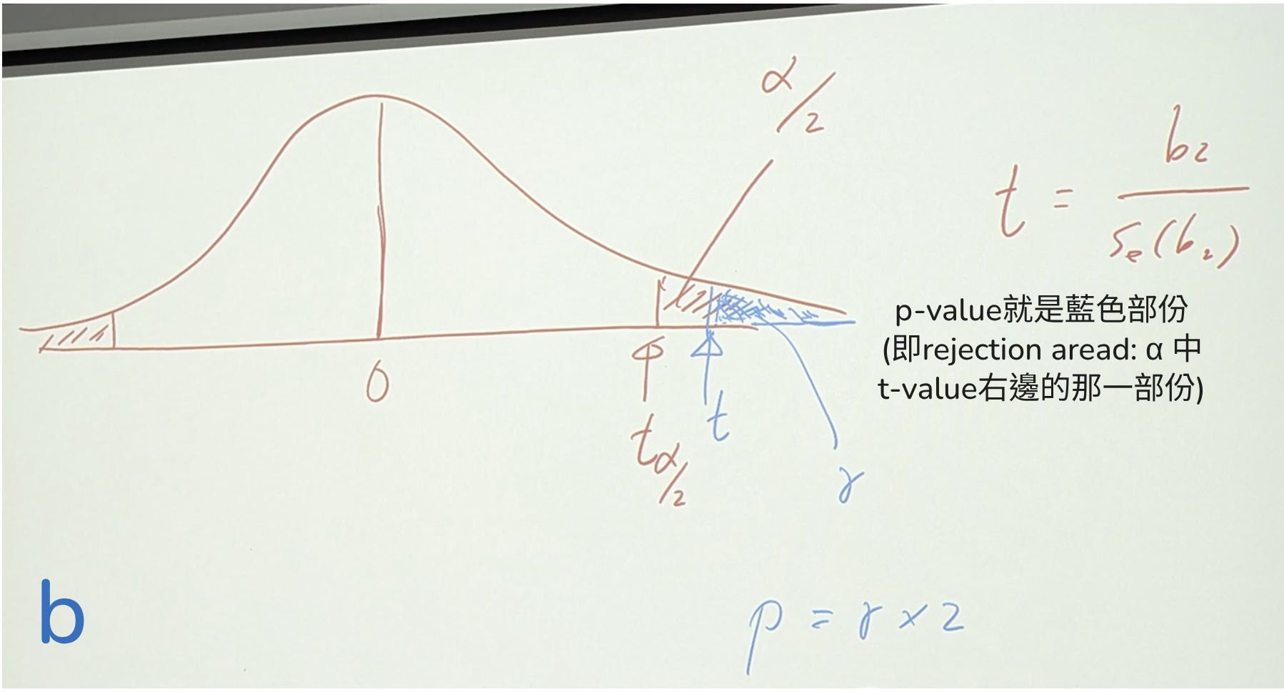
(圖b)
比如(表1)
那個C的p-value(Prob.)=0.0622,明顯就比0.05(假如是95%單尾)還大,明顯就是insignificant。Not reject。
而INCOME的p-value(Prob.)=0.0000,明顯就小於0.05甚至於比0.01,0.001都小,一看就知道是significant應該要reject Null Hyothesis。
所以說,有p-value可看時,一般就不用去查tc值來和t值比對,可以快速做出判斷。
這就是用food.wf1 看整個過程的詳細解說
★ Normally Hypothesis alternative allways one you belive, and H-null is one you want to reject!
p.124 [EXAMPLE 3.3 Right-Tail Test of an Economic Hypothesis 經濟假設的右尾檢驗]
這就是用food.wf1 看整個過程的詳細解說
現在,我們要根據收集到的40個(收入-食物支出)樣本進行推估,並提出可信服的證明給總經理做決策參考!
考量: 雖然說β2的最小平方法估計值為b2=10.21,大於5.5。但我們想要確定的是,是否有令人信服的統計證據能夠讓我們基於現有數據得出 β2>5.5的結論。這項判斷不僅基於估計值b2,還要基於其精確度(以 se(b2) 來衡量)。
2.指定檢定統計量及其分佈。
- 統計量 t=(b2-C) / se(b2) =(b2- 5.5) / se(b2) ~t(N-2) 。(若null hypothesis為真)
3.設信賴區間的 α = 0.01。
- 右尾拒絕域的臨界值是自由度為N-2=38的t分佈的第99個百分位數,即 t(0.99, 38)=2.429。如果計算出的t值≥2.429,我們將拒絕原假設。(反之: 如果t<2.429,我們將不拒絕原假設。)
4.經Eviews計算-得到b2=10.21 和 se(b2)= 2.09 所以, t=(b2-5.5) / se(b2) = (10.21-5.5)/2.09 =2.25(或 P-value=nn.nn) 。
5.因為 t = 2.25 < 2.429, 不在拒絕域中,所以不能拒絕null hypothesis H0 (即β2 ≤ 5.5)。
結論:
We are not able to conclude that the new supermarket will be profitable and will not begin construction.
(在每種現實情況下,必須根據風險評估和做出錯誤決策的後果來選擇 α,像此處就採取更嚴格的要求0.01)。
▼Eviews8.1操作法 (Wald Test 省心好辦法!)
如果是用Eviews(不必手算),這樣做
如果是用Eviews(不必手算),這樣做:
EX3.3-a: 使用food.wf1檔: Quick > Estimae Equation > food_exp c income
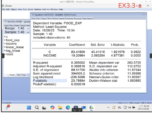
EX3.3-b: View > Coefficient Diagnostics > Wald Test-Coefficient Restirctions..
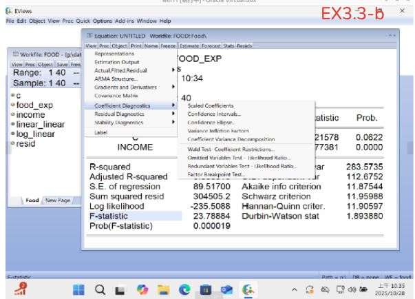
EX3.3-c: 輸入c(2)=5.5 > OK
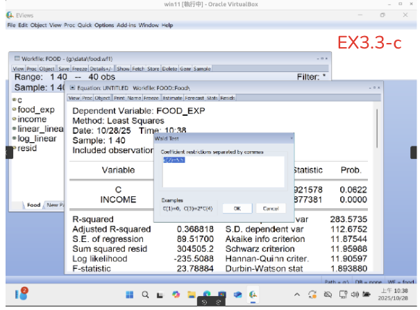
EX3.3-d: 幫你算好t-statistic=2.249904 及p-value=0.0303 (因為要求是0.01 所以fail to reject)
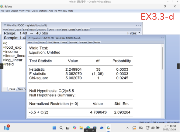
Wald-test的 c(2)其實就是 c去幫你減掉c(2)這個值 的意思。
這裡要教用view -> Cofeficcient Dignostics -> Wald-test: c(2)=5.5 -> OK
restrictions separated by commas (公式只能用 =) 請輸入
做出t-statistic 0.0303
???? 因為是2 tails所以要 0.0303/2= 0.015 比 0.01還要大 所以不能reject
*****這部份要小心 好好利用Wald-test 須搞清楚,one tail 或two
tails***會很好用!!
這兩個案例很重要,詳細做過,就了解了!!
會影響準確度有兩個因素 1.是confidence level; 2.是se(b2)-這可去看interval(分散程度)
這是簡單的例子,但其中有很多需要深思的意義。
p.125 [EXAMPLE 3.4 Left-Tail Test of an Economic Hypothesis 經濟假設的左尾檢驗]
看看他是怎樣算出結果 和如何reject null 的
為了完整起見,這裡有個(拒絕域在左尾部)的示範。我們考慮H0虛無假設 β2 ≥ 15 且備擇假設 β2 < 15。
1.Determine the null and alternative hypotheses:
設定H0: β2 ≥ 15 ,和H1: β2 < 15。
2.Specify the test statistic and its distribution if the null hypothesis is true:指定檢定統計量及其分佈:
- 統計量 t=(b2-C) / se(b2) (若null hypothesis為真)。
設信賴區間的 α = 0.05 :
- 左尾拒絕域的臨界值是自由度為N-2=38的t分佈的第5個百分位數,即 t(0.95, 38)=−1.686。如果計算出的t值≤ −1.686,我們將拒絕原假設。(反之: 如果t>−1.686,我們將不拒絕原假設。)
經Eviews計算-得知 b2=10.21 和 se(b2)= 2.09 所以,
t=(b2 - 15) / se(b2) = (10.21-15)/2.09 = -2.29
P-value=nn.nn。
結論:
由於 t = −2.29 < −1.686,我們拒絕虛無假設β2≥15,接受備擇假設β2 <15。我們得出結論,家庭每增加100美元收入,在食物上的支出不到15美元。
p.125 [EXAMPLE 3.5 Two-Tail Test of an Economic Hypothesis 經濟假設的雙尾檢驗]
注意5.Since -2.204是課本寫錯了! 應該是2.024才對 他左下的tcritical處2.024是正確的。
請看:這也是個例子 Se如過大(sample不夠多(重新取樣或或取更多sample),或是,模型只用一條簡單的回歸線是不正確的),會影響判斷結果。
某顧問認為,根據其他類似社區的情況,擬建市場附近的家庭每增加100美元收入,就會額外支出7.50美元。根據我們的經濟模型,我們可以將這個猜想表述為零假設: β2 = 7.5。如果我們想檢驗這個假設是否成立,則備擇假設是 β2 ≠ 7.5。此備擇假設並未明確 β2是大於7.5或小於7.5,但顯示它不是7.5。在這種情況下,我們就應使用雙尾檢驗,過程如下。
1.Determine the null and alternative hypotheses:
設定H0: β2 = 7.5,和H1: β2 ≠ 7.5。
2.Specify the test statistic and its distribution if the null hypothesis is true:指定檢定統計量及其分佈。
- 統計量 t=(b2-C) / se(b2) (若null hypothesis為真),所以應該是:
t=(b2 - 7.5) / se(b2)
。
設信賴區間為95% 也就是設定 α = 0.05, 那意思就是在兩個尾端各有2.5%的拒絕域。
因此兩個t-critical value分別是位在第2.5-percentile t(0.025, 38) = −2.024 和第97.5-percentile t(0.975, 38) = 2.024 的點上。
經Eviews計算-得到b2=10.21 和 se(b2)= 2.09 所以,
t=(b2 -c) / se(b2) = (10.21 -7.5) / 2.09 = 1.29 或
P-value=nn.nn。
結論:
這樣看來: –2.024 < t = 1.29 < 2.024,因此不能拒絕 H0=7.5 的虛無假設null hypothesis。 So that
our conclussion is "The sample data are consistent with the conjecture households will spend an additional $7.50 per additional $100 income on food."
也就是說:“樣本數據與以下推測一致:家庭每增加 100 美元收入就會在食品上多花費 7.50 美元。”
必須避免過度解讀這個結論。這並非從此檢定得出β2 = 7.5的結論,而只是顯示數據與該參數值並非不相容。這數據也與虛無假設H0∶β2 = 8.5(t = 0.82)或 H0∶β2 = 6.5(t = 1.77)甚至於H0∶β2 = 12.5(t = −1.09)都相容。
換句話說:假設檢定不能用來證明零假設成立,只是 不能推翻not reject。
你可能注意到了這個小技巧: 設q=100(1 − α)%
bk − tc se(bk) ≤ q ≤ bk + tc se(bk)
我們不主張使用信賴區間來檢驗假設,它們有不同的用途,但如果給定信賴區間,這個技巧就很方便。
besides, “Statistically significant” does not necessarily imply “economically significant.”
3.5 The p-Value
規則很簡單:當if p ≤ α, 就拒絕H0. 反之若 p > α, 就不能拒絕 do not reject H0 (參考上面的圖b).
p-value 其實就是: cumulative distribution function (cdf) (see Appendix B.1)
要精確計算的公式與過程是基於學生t分佈Student's t-distribution的累積機率函數Cumulative Distribution Function, CDF或其補數生存函數Survival Function, SF來進行的。
1.「精確計算」的公式在雙尾檢定Two-Tailed Test中,給定t統計量t_stat和自由度df,計算p值的通用公式為:
p-value = 2 * P(T > |tstat| with df)
其中: (以下是用到W07的作業2-b問題的內容)
|tstat|:是t統計量的絕對值,因為是雙尾檢定,我們考慮正負兩個方向的極端值。P(T > |tstat| with df):表示在自由度為df的t分佈下,隨機變數T大於|tstat|的機率,即t分佈曲線右側尾部的面積。
2 *:由於是雙尾檢定,必須將單一尾部面積乘以兩倍,以涵蓋T>3.199和T<-3.199兩側的極端機率。
個計算通常無法透過手動查表精確得到,而是依賴於統計軟體或程式庫中的數值積分。在 Python 的 SciPy 程式庫中,這個過程使用以下函數實現:Tail Area = scipy.stats.t.sf(|tstat|, df)
sf (Survival Function) 即1-CDF,它直接計算T大於tstat的機率。
若用bash程式執行方式是: htw@htwnb:~$ python3 htw_p_value_calculator.py
p.126 [EXAMPLE 3.6 Two-Tail Test of Significance 雙尾顯著性檢定]
For Econometrics, normally use this 3 tests: t-test of F-test or Chi-square-test
1.Determine the null and alternative hypotheses:
設定H0: β2 <= [??],和H1: β2 > [??]。
2.Specify the test statistic and its distribution if the null hypothesis is true:指定檢定統計量及其分佈。
- 統計量 t=(b2-C) / se(b2) (若null hypothesis為真),所以應該是:
t=(b2 - 7.5) / se(b2)
。
設信賴區間的 α = 0.01/0.05 ?。
4.Calculate the sample value of the test statistic:經Eviews計算-得到b2=ww.ww 和 se(b2)= zz.zz 所以,
t=b2 / se(b2) = ww.ww/zz.zz =[??] 或
P-value=nn.nn。
結論:
....
p.129 [3.6 Linear Combinations of Parameters]
簡單明瞭TileStatsLinear regression | hypothesis testing
t=(b1+2b2-5)/Se(b1+2b2)
Var(c1b1+c2b2) = var(λ)
covariance matrix 就是
view coe diag wal-test > hypo null 公式: c(1)+2*c(2)=5
你可以把Se 39.476 平方就是variance
var(b1)= 188 var(b2)=4.38
p.130 [EXAMPLE 3.7 Estimating Expected Food Expenditure]
這個例子就是 [3.6 Linear Combinations of Parameters]
這個沒有做什麼test
下個例子,是做出 interval estimate
p.131 [EXAMPLE 3.8 An Interval Estimate of Expected Food Expenditure]
這個計算需要先找出 se(c1b1+c2b2)
view -> Cofeficcient Dignostics -> Wald-test: hypo null 公式:
c(1)+2c(2)=5
c(1)+20c(2)=(任何number: 因為只是想找出se 就是 14.178
p.132 [EXAMPLE 3.9 Testing Expected Food Expenditure] “I expect that a household with $2,000 weekly income will spend, on average, more than $250 a week on food.” How can we use econometrics to test this conjecture?
也是view -> Cofeficcient Dignostics -> Wald-test: c(1)+20*c(2)=250
p.140 3.21 The capital asset pricing model (CAPM) is described in Exercise 2.16. Use all available observations in the data file capm5 for this exercise.
▼作業2 Asigment_2
[p.140] 3.21 The capital asset pricing model (CAPM) is described in Exercise 2.16. Use all available observations in the data file capm5 for this exercise.
a. Construct 95% interval estimates of Exxon-Mobil’s and Microsoft’s “beta.” Assume that you are a stockbroker. Explain these results to an investor who has come to you for advice.
b. Test at the 5% level of significance the hypothesis that Ford’s “beta” value is one against the alternative that it is not equal to one. What is the economic interpretation of a beta equal to one? Repeat the test and state your conclusions for General Electric’s stock and Exxon-Mobil’s stock. Clearly state the test statistic used and the rejection region for each test, and compute the p-value.
c. Test at the 5% level of significance the null hypothesis that Exxon-Mobil’s “beta” value is greater than or equal to one against the alternative that it is less than one. Clearly state the test statistic used and the rejection region for each test, and compute the p-value. What is the economic interpretation
of a beta less than one?
d. Test at the 5% level of significance the null hypothesis that Microsoft’s “beta” value is less than or equal to one against the alternative that it is greater than one. Clearly state the test statistic used and the rejection region for each test, and compute the p-value. What is the economic interpretation of a beta more than one?
e. Test at the 5% significance level, the null hypothesis that the intercept term in the CAPM model for Ford’s stock is zero, against the alternative that it is not. What do you conclude? Repeat the test and state your conclusions for General Electric’s stock and Exxon-Mobil’s stock. Clearly state the test statistic used and the rejection region for each test, and compute the p-value.
Hypothesis Testing: α = 0.05; H0: β(mkt_rf)=1 ; H1: β(mkt_rf)≠1;
equation estiamate: ford_rf c mkt_rf (by Eviews get answer:)
MKT_RF: β=1.662031 se=0.206937 t-value=8.031573 p-value=0.0000
(注意:這裡的t-Statistic=t-value 8.031573 是根據β(mkt_rf)=0 計算出來的)
t-value=(1.662031 - 1) /0.206937= 3.199 > t(0.025,178) = 2.024
且 p-value=0.0000 所以應reject H0: β(mkt_rf)=1 ,結論是 β(mkt_rf)≠1
(同樣方法再去做 General Electric’s stock and Exxon-Mobil’s stock.)
答c: Exxon-Mobil's stock (這是左尾檢定)
Hypothesis Testing: α = 0.05; H0: β(mkt_rf)≥1 ; H1: β(mkt_rf)<1;
equation estiamate: xom_rf c mkt_rf (by Eviews get answer:)
MKT_RF: β=0.456521 se=0.071550 t-value=6.380428 p-value=0.0000
(注意:這裡的t-Statistic=t-value 6.380428 是根據β(mkt_rf)=0 計算出來的)
t-value=(0.456521 - 1) /0.071550= -7.596 < t(0.95,178) = -1.686
且 p-value=0.0000 所以應reject H0: β(mkt_rf)<1 ,結論是 β(mkt_rf)<1
答d: Microsoft's stock (這是右尾檢定)
Hypothesis Testing: α = 0.05; H0: β(mkt_rf)≤1 ; H1: β(mkt_rf)>1;
equation estiamate: msft_rf c mkt_rf (by Eviews get answer:)
MKT_RF: β=1.201840 se=0.122152 t-value=9.838921 p-value=0.0000
(注意:這裡的t-Statistic=t-value 9.838921 是根據β(mkt_rf)=0 計算出來的)
t-value=(1.201840 - 1) /0.122152= 1.6523 < tc(0.95,178) = 1.6535
且 p-value= 0.050118 所以應not reject H0: β(mkt_rf)≤1 ,結論是 β(mkt_rf)≤1
答e: Ford's stock (這是右尾檢定)
Hypothesis Testing: α = 0.05; H0: α(mkt_rf)=0 ; H1: α(mkt_rf)≠0;
equation estiamate: ford_rf c mkt_rf (by Eviews get answer:)
Intercept: C=0.003779 se=0.010225 t-value=0.369564 p-value=0.7121
且 p-value=0.7121 所以應not reject H0: α(mkt_rf)=0; ,結論是α(mkt_rf)=0
A:在命令視窗: 輸入指令 genr msft_rf = msft - riskfree
genr 是generate series生成數列的縮寫。
msft_rf 是想建立的新變數名稱。
msft - riskfree 是計算公式。
執行:按下鍵盤上的 Enter 鍵。
執行後,工作檔列表Workfile window中會多出一個新的數列變數MSFT_RF出現。
下週講Chp04 Prediction, Goodness-of-Fit, and Modeling Issues
老師會跳過Prediction因為有其他工具可用(有興趣可自學),只講後面的Goodness-of-Fit,
and Modeling Issues
就是講義4.2-4.6
W08 Chp04 Prediction, Goodness-of-Fit, and Modeling Issues
2025-10-29-Tuesday 14:00-17:00 林師模教授 (換到402A教室)
課本: Principles of Econometrics, 5th Edition | Chp04 第152頁開始。
講義: Ch-04 Prediction, Goodness-of-Fit, and Modeling Issues
▼Goal of Chp04
Based on the material in this chapter, you should be able to
1.Explain how to use the simple linear regression model to predict the value of y for a given value of x.解釋如何使用簡單線性迴歸模型預測給定 x 值時 y 的值。
2.Explain, intuitively and technically, why predictions for x values further from x are less reliable.
從直覺和技術層面解釋為什麼 x 值偏離 x 值越遠,預測的可靠性越低。
3.Explain the meaning of SST, SSR, and SSE, and how they are related to R2.
解釋 SST、SSR 和 SSE 的意義,以及它們與 R2 的關係。
4.Define and explain the meaning of the coefficient of determination.
定義並解釋判定係數的涵義。
5.Explain the relationship between correlation analysis and R2.
解釋相關性分析與 R2 之間的關係。
6.Report the results of a fitted regression equation in such a way that confidence intervals and hypothesis tests for the unknown coefficients can be constructed quickly and easily.
報告擬合迴歸方程式的結果,以便能夠快速輕鬆地建立未知係數的置信區間和假設檢定。
7.Describe how estimated coefficients and other quantities from a regression equation will change when the variables are scaled. Why would you want to scale the variables?
描述迴歸方程式中估計的係數和其他量在變數縮放後會如何變化。為什麼要縮放變數?
8.Appreciate the wide range of nonlinear functions that can be estimated using a model that is linear in the parameters.
理解可以使用參數線性的模型來估計各種非線性函數。
9.Write down the equations for the log-log, log-linear, and linear-log functional forms.
寫出對數-對數、對數-線性和線性-對數函數形式的方程式。
10.Explain the difference between the slope of a functional form and the elasticity from a functional form.
解釋函數形式的斜率與函數形式的彈性之間的差異。
11.Explain how you would go about choosing a functional form and deciding that a functional form is adequate.
解釋如何選擇函數形式並確定其是否合適。
12.Explain how to test whether the equation ‘‘errors’’ are normally distributed.
解釋如何檢定方程式的「誤差」是否服從常態分佈。
13.Explain how to compute a prediction, a prediction interval, and a goodness-of-fit measure in a log-linear model.
解釋如何在對數線性模型中計算預測值、預測區間和適合度。
14.Explain alternative methods for detecting unusual, extreme, or incorrect data values.
解釋檢測異常、極端或不正確資料值的其他方法。
李柏融 卡方檢定
卡方檢定的觀念 數量資料(母數統計)-類別資料(無母數統計)>卡方主要做類別資料檢定:(觀察值-期望值)的平方/期望值=Chi square值。
Goodness-of-Fit Test ▶️適合度檢定(常態分配檢定例題),例:公正骰子,電瓶壽命。
Independent Test ▶️獨立性檢定注意,自由度是df=(r-1)(c-1),例:宗教信仰與區域性無關
Homogeneity Test ▶️齊一性檢定目的:檢定兩個或兩個以上的母體某一特性的分配是否相同或相近?注意,自由度是df=(r-1)(c-1),兩種不同肥料使發芽率是否一樣
- Examining the correlation between sample values of y and their predicted values provides a goodness-of-fit measure called R2 that describes how well our model fits the data. 檢查 y 的樣本值與其預測值之間的相關性,可以提供適合度測量(稱為 R2),該測量描述了我們的模型與資料的適合程度。 - For each observation in the sample, the difference between the predicted value of y and the actual value is a residual. Diagnostic measures constructed from the residuals allow us to check the adequacy of the functional form used in the regression analysis and give us some indication of the validity of the regression assumptions. 對於樣本中的每個觀測值,y 的預測值與實際值之間的差異就是殘差。基於殘差建構的診斷指標使我們能夠檢查迴歸分析中使用的函數形式的充分性,並在一定程度上表明迴歸假設的有效性。 - We will examine each of these ideas and concepts in turn.
p.153 [4.1 Least Squares Prediction]
p.156 [4.2 Measuring Goodness-of-Fit 配適度測量(R2) 測量擬合優度]
當我們要估計或檢定常態變數的「變異數」,時必須用到卡方分配。
(n-1)s2/σ2 服從自由度(n-1)的卡方分配,也就是 (n-1)s2/σ2 ~ χ2
χ2 = Σ(i=1,n) (Oi-Ei)2 / Ei
以上說的是卡方分配的Goodness-of-Fit; 但這裡要談的是
SST= total sum of squares
SSR= sum of squares due to the regression
SSE= sum of squares due to error
SST= SSR + SSE
R2=SSR/SST = 1-(SSE/SST)
p.159 [EXAMPLE 4.2 Goodness-of-Fit in the Food Expenditure Model]
- 請參考p.63 的[EXAMPLE 2.4a Estimates for the Food Expenditure Function]
b2 = Σ(xi-xbar)(yi-ybar)/Σ(xi-xbar)2 = SSxy / SSxx; (而b1= ybar - b2xbar)
因為: R2 = SSR/SST = 1-(SSE/SST)
這個 SSE 就是寫在 Sum squared resid (304505.2)
這個 SST 則須要拿 S.D. dependet var (112.6752) 來計算
因為公式 σ2 = Σ(y-ybar)^2 / (n-1) df = SST / (n-1) df
所以公式可代換成 SST = σ2 * (n-1)
已知
S.D. dependet var (112.6752) 這就是 σ
(n-1) = 40-1 =39 (因為n是樣本數40)
所以 SST = (112.6752)2 39 = 495130.569
因此: R2 = 1-(SSE/SST) = 1-(304505.2 / 495130.569) = 1-0.61 = 0.39 (就是這樣算出來的!)
目前只有39%的(R-squared) Goodness-fit of the line, 所以可能要換Modelshap!!
p.157 [4.2.1 Correlation Analysis]
(Ρ大寫,ρ小寫/ˈroʊ/) ρxy The correlation coefficient between x and y is defined in (B.21) -p.773ρxy = σxy / σxσy
rxy = sxy / sxsy
p.158 [4.2.2 Correlation Analysis and R2]
用Eviews怎樣算出 correlation coefficent (圖片)
選food_exp +Ctrl incomme > Open as group > View > Covarance Analysis > Correlation打勾 >OK
可以看到 food_exp和incomme 的correlation r= 0.620485
為了確認,驗算 r2 = 0.6204852 = 0.3805002 = R2 沒錯。
- Asterisks are often used to show the reader the statistically significant (i.e., significantly different from zero using a two-tail test) coefficients, with explanations in a table footnote:
* indicates significant at the 10% level
** indicates significant at the 5% level
*** indicates significant at the 1% level
寫法如下:
FOOD_EXP = 83.42 + 10.21 INCOME R<sup<2> = 0.385002
(sd) (43.41)* (2.09)***
(t) (1.92)* (4.88)***
p.160 [4.3 Modeling Issues]
p.160 [4.3.1 The Effects of Scaling the Data 數據規模的影響]
- a change in the units of measurement is called scaling the data.增減x或y 的單位,不會影響R2和 sd。
p.161 [4.3.2 Choosing a Functional Form]
- quadratic and log-linear functional forms二次和對數線性函數形式1. Power: If x is a variable, then xp means raising the variable to the power p; examples are quadratic (x2) and cubic (x3) transformations.
2. The natural logarithm: If x is a variable, then its natural logarithm is ln(x).
- Using just these two algebraic transformations, there are amazing varieties of “shapes” that we can represent, as shown in Figure 4.5.
(圖)
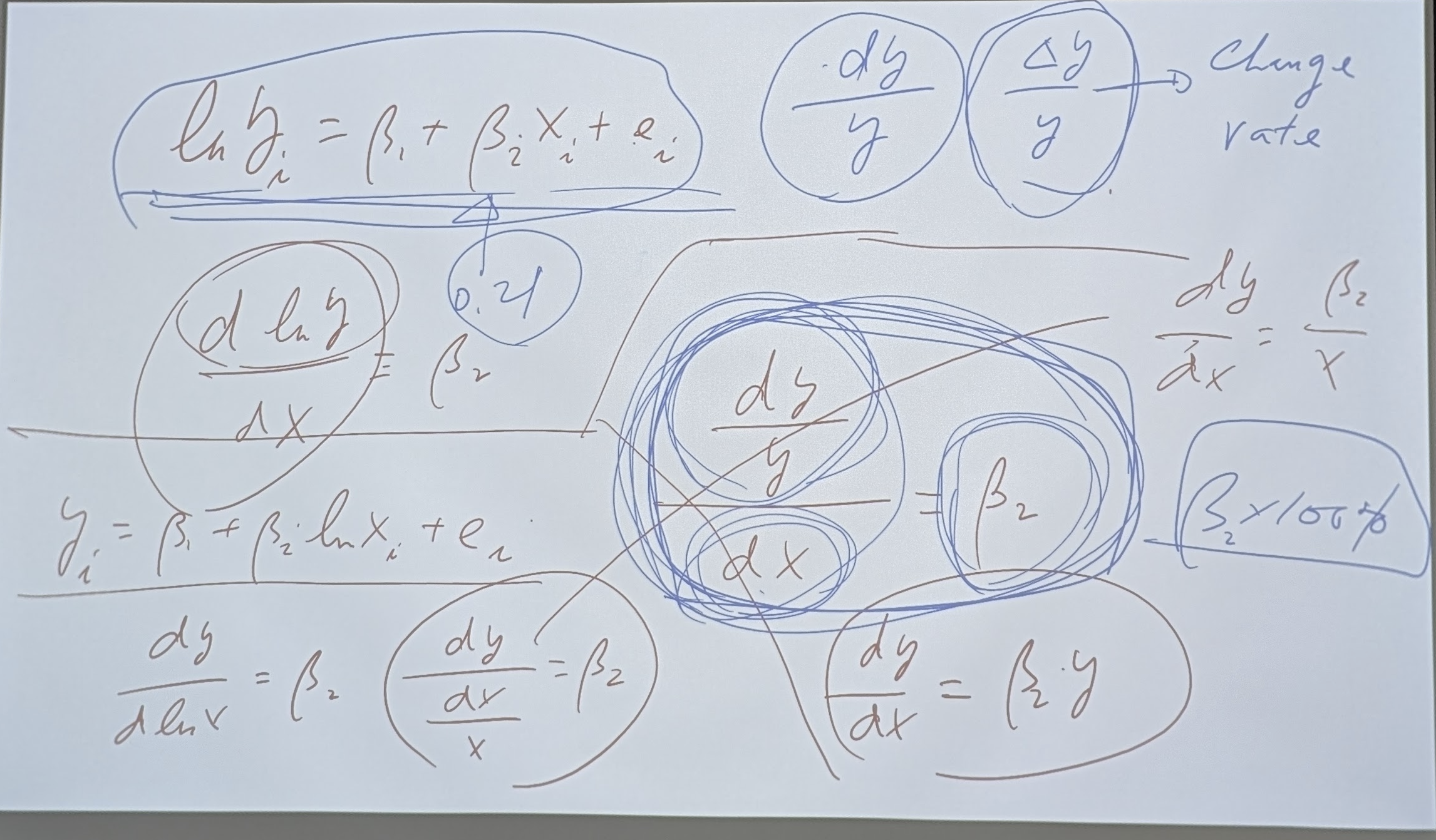
- elasticity change彈性變化,deviation 偏差
- 有時需要用到Quadratic 或exponatial function 可能更加better fit the regression line
所謂Quadratic 是把x squared 成為 x2; 又或許可以x不變,但是ln(y) -natural log(y)
TABLE 4.1 -Some Useful Functions, Their Derivatives, Elasticities, and Other Interpretation一些有用的函數、它們的導數、彈性及其他解釋
(回頭看p.79 的EXAMPLE 2.6 Baton Rouge House Data -這裡有計算elasticities的說明)
p.64有解釋: Elasticities還有公式和實例。
yi=β1+β2 +ei => dy/dx = β2 = marginal effect
yi=β1+β2 x2+ei=> dy/dx = 2 β2 x2 (如果x改為x2的話)
注意 dy/dx 的interpret, 也就是他在變動時,所代表的意義!
log > focast >
d ln(y) / d ln(x) = (dy/y) / (dx/x) = (dy/dx)(x/y) = 看需求的價格彈性Price elasticity of demand 公式; = β2 (x/y) 看p.163 TABLE4.1 的founction of Linear就是這個意思。
Slope= dy/dx = β2 so that: = β2 (x/y)
(看p.178 EXAMPLE 4.13 The log-log functional form is frequently used for demand equations.)
• 當 彈性 > 1 時,表示應變數對自變數的變化非常敏感,即自變數變化1%會導致應變數變化超過1%。這種情況稱為高彈性或富有彈性。
• 當 彈性 < 1 時,表示應變數對自變數的變化不太敏感,即自變數變化1%會導致應變數變化少於1%。這種情況稱為低彈性或缺乏彈性。
舉個例子,如果在一個需求模型中,價格彈性為0.5,這意味著價格上升1%會導致需求下降0.5%。相反,如果價格彈性為1.5,價格上升1%會導致需求下降1.5%。
W09 --期中考--
2025-11-05-Tuesday 14:00-17:00 林師模教授
W10 Chp04 Prediction, Goodness-of-Fit, and Modeling Issues
2025-11-12-Tuesday 14:00-17:00 林師模教授
課本: Principles of Econometrics, 5th Edition |
講義: Ch-04 Prediction, Goodness-of-Fit, and Modeling Issues
p.163 [4.3.3 A Linear-Log Food Expenditure Model]
TABLE4.1 是一些有用的函數、它們的導數、彈性及其他解釋。Some Useful Functions, Their Derivatives,Elasticities, and OtherInterpretation這是濟學中迴歸模型(Regression Models)與彈性分析(Elasticity Analysis)的核心觀念之一: 這五種常見模型的**函數形式、導數(邊際效果)、彈性公式、以及典型的經濟學應用理論**:
1.Linear Model(線性模型)
導數(marginal effect)=(dy/dx);
彈性Elasticity =(dy/dx)(x/y); 典型應用:
消費函數(Consumption Function):C = a + bYd,其中邊際消費傾向(MPC)為常數。
成本函數(Cost Function):總成本與產量呈線性增長的簡化模型。
2.Quadratic Model(二次模型) 導數:(dy/dx)=β1 + 2β2X ;
彈性:E=(β1+2β2X)⋅(X/Y) ;
典型應用: 生產函數(Production Function)中遞減報酬理論(Law of Diminishing Returns)。
3.Cubic Model(三次模型) 導數:(dy/dx)=β1+2β2X+3β3X2 可捕捉多重轉折(例如 S 形曲線)。
彈性:E=(β1+2β2X+3β3X2)⋅(X/Y)
典型應用:學習曲線、技術擴散曲線、或市場成長
的「S形」現象。
初期緩慢、中期加速、後期趨緩。
總成本或報酬曲線存在多個階段的情形。
4.Log-linear Model(半對數模型)
導數:(dy/dx)=β2⋅Y (邊際效果隨 Y 成比例變化)。
彈性:E=
典型應用:經驗曲線(Experience Curve):成本隨產量呈指數下降。
Phillips Curve(通脹與失業率關係)等非線性現象。
成長模型中呈現「相對變化率固定」的現象。
5.Log-log Model(對數-對數模型,常稱「雙對數模型」)
導數:(dy/dx)= β2 (y/x)
彈性:E=β2
典型應用:需求函數(Demand Function): 即為價格彈性。
生產函數(Cobb-Douglas Production Function):
規模報酬(Returns to Scale)分析: → 常報酬。
p.192 [Appendix]
Appendix 4A Development of a Prediction Interval 預測區間的建立Appendix 4B The Sum of Squares Decomposition 平方和分解
Appendix 4C Mean Squared Error: Estimation and Prediction 均方誤差:估計與預測
▼ Assignment3題目與之前的作業題參考
Fair’s data, 26 observations for the election years from 1916 to 2016, are in the data file fair5. The dependent variable is
VOTE = percentage share of the popular vote won by the Democratic Party. Consider the effect of economic growth on VOTE.
If Democrats are the incumbent party (INCUMB = 1) then economic growth, the growth rate in real per capita GDP in the first three quarters of the election year (annual rate), should enhance their chances of winning. On the other hand,
if the Republicans are the incumbent party (INCUMB = −1), growth will diminish the Democrats’ chances of winning. Consequently, we define the explanatory variable GROWTH = INCUMB × growth rate.
Using the data for 1916–2012, plot a scatter diagram of VOTE against GROWTH. Does there appear to be a positive association?
Estimate the regression VOTE = β1 + β2GROWTH + e by least squares using the data from 1916 to 2012. Report and discuss the estimation result. Plot the fitted line on the scatter diagram from (a).
Using the model estimated in (b), predict the 2016 value of VOTE based on the actual 2016 value for GROWTH. How does the predicted vote for 2016 compare to the actual result?
Economy wide inflation may spell doom for the incumbent party in an election. The variable INFLAT = INCUMB × inflation rate, where the inflation rate is the growth in prices over the first 15 quarters of an administration. Using the data from 1916 to 2012, plot VOTE against INFLAT.
Using the data from 1916 to 2012, report and discuss the estimation results for the model VOTE = α1 + α2INFLAT + e.
Using the model estimated in (e), predict the 2016 value of VOTE based on the actual 2012 value for INFLAT. How does the predicted vote for 2016 compare to the actual result?
[p.141] 3.24 We introduced Professor Ray C. Fair’s model for
explaining and predicting U.S. presidential elections in Exercise 2.23.
Fair’s data, 26 observations for the election years from 1916 to 2016,
are in the data file fair5. The dependent variable is VOTE =
percentage share of the popular vote won by the Democratic party. Define
GROWTH = INCUMB × growth rate, where growth rate is the annual rate of
change in real per capita GDP in the first three quarters of the
election year. If Democrats are the incumbent party, then INCUMB = 1; if
the Republicans are the incumbent party then INCUMB = −1.
Estimate the linear regression, VOTE = β1 + β2GROWTH + e, using data from 1916 to 2016. Construct a 95% interval estimate of the effect of economic growth on expected VOTE. How would you describe your finding to a general audience?
The expected VOTE in favor of the Democratic candidate is E(VOTE|GROWTH) = β1 + β2GROWTH. Estimate E(VOTE|GROWTH = 4) and construct a 95% interval estimate and a 99% interval estimate. Assume a Democratic incumbent is a candidate for a second presidential term. Is achieving a 4% growth rate enough to ensure a victory? Explain.
Test the hypothesis that when INCUMB = 1 economic growth has either a zero or negative effect on expected VOTE against the alternative that economic growth has a positive effect on expected VOTE. Use the 1% level of significance. Clearly state the test statistic used, the rejection region, and the test p-value. What do you conclude?
Define INFLAT = INCUMB × inflation rate, where the inflation rate is the growth in prices over the first 15 quarters of an administration. Using the data from 1916 to 2016, and the model VOTE = α1 + α2INFLAT + e, test the hypothesis that inflation has no effect against the alternative that it does have an effect. Use the 1% level of significance. State the test statistic used, the rejection region, and the test p-value and state your conclusion.
4.24 Reconsider the presidential voting data (fair5) introduced in
Exercises 2.23 and 3.24.
Using all the data from 1916 to 2012, estimate the regression model VOTE = β1 + β2GROWTH + e. Based on these estimates, what is the predicted value of VOTE in favor of the Democrats in 2012? At the time of the election, a Democrat, Barack Obama, was the incumbent. What is the least squares residual for the 2012 election observation?
Estimate the regression in (a) using only data up to 2008. Predict the value of VOTE in 2012 using the actual value of GROWTH for 2012, which was 1.03%. What is the prediction error in this forecast? Is it larger or smaller than the error computed in part (a).
Using the regression results from (b), construct a 95% prediction interval for the 2012 value of VOTE using the actual value of GROWTH = 1.03%.
Using the estimation results in (b), what value of GROWTH would have led to a prediction that the nonincumbent party [Republicans] would have won 50.1% of the vote in 2012?
Use the estimates from part (a), and predict the percentage vote in favor of the Democratic candidate in 2016. At the time of the election, a Democrat, Barack Obama, was the incumbent. Choose several values for GROWTH that represent both pessimistic and optimistic values for 2016. Cite the source of your chosen values for GROWTH.
W11 --本週課目標題--
2025-11-19-Tuesday 14:00-17:00 林師模教授
- 因承辦2025合經同學會,請假!
Chp05只講一半還沒有講完
【谷哥統計】第09單元:多元迴歸分析Multiple regression analysis 40:00
高斯-馬可夫定理Gauss–Markov theorem陳述的是在線性迴歸模型中,如果線性模型滿足高斯馬可夫假定,則迴歸係數的「最佳線性不偏估計」就是普通最小平方法估計。最佳估計是指相較於其他估計量有更小變異數的估計量,同時把對估計量的尋找限制在所有可能的線性不偏估計量BLUE中。此外,誤差也不一定需要滿足獨立同分布或常態分布。
國語版
Gauss Markov Theorem: Slope Estimator is Unbiased
W12 Chp05 The Multiple Regression Model
2025-11-26-Tuesday 14:00-17:00 林師模教授
課本: Principles of Econometrics, 5th Edition [P.196] |
講義: Ch-05 Prediction, Goodness-of-Fit, and Modeling Issues
- 今日因宜安轉台北榮總-請假沒上課;
- 珮彤說:今天3人請假,沒有作業,下次從第六章開始教。且今天學校Eviews當機,所以老師沒有示範eview怎麼作,下週會示範給大家看。
W13 Chapter 6 Further Inference in the Multiple Regression Model
2025-12-03-Tuesday 14:00-17:00 林師模教授
課本: Principles of Econometrics, 5th Edition [P.260] |
講義: Ch-06 Further Inference in the Multiple Regression Model
6.2 The F-Test Procedure
1. Specify the null and alternative hypotheses: The joint null hypothesis is H0∶β3 = 0, β4 = 0. The alternative hypothesis is H1∶β3 ≠ 0 or β4 ≠ 0 or both are nonzero.
2. Specify the test statistic and its distribution if the null hypothesis is true: Having two restrictions in H0 means J = 2. Also, recall that N = 75, so the distribution of the F-test statistic when H0 is true is
3. Set the significance level and determine the rejection region: Using α = 0.05, the critical value from the F(2, 71)-distribution is Fc = F(0.95, 2, 71), giving a rejection region of F ≥ 3.126. Alternatively, H0 is rejected if p-value ≤ 0.05.
4. Calculate the sample value of the test statistic and, if desired, the p-value: The value of the F-test statistic is The corresponding p-value is p = P(F(2, 71) > 8.44)=0.0005.
5. State your conclusion: Since F = 8.44 > Fc = 3.126, we reject the null hypothesis that both β3 = 0 and β4 = 0, and conclude that at least one of them is not zero. Advertising does have a significant effect upon sales revenue. The same conclusion is reached by noting that p-value = 0.0005 < 0.05.
You might ask where the value Fc = F(0.95, 2, 71) = 3.126 came from. The F critical values in Statistical Tables 4 and 5 are reported for only a limited number of degrees of freedom. However, exact critical values such as the one for this problem can be obtained for any number of degrees of freedom using your econometric software.
Remark
The usual F-test of a joint hypothesis relies on
the assumptions MR1–MR6 of the linear regression model. Of particular
relevance for testing the equivalence of two regressions is assumption
MR3, that the variance of the error term, var(ei|)= σ2, is the same for
allobservations.
If we are considering possibly different slopes and intercepts for parts
of the data, it might also be true that the error variances are
different in the two parts of the data.
In such a case, the usual F-test is not valid. Testing for equal
variances is covered in Section 8.2, and the question of pooling in this
case is covered in Section 8.4. For now, be aware that we are assuming
constant error variances in the calculations above.
老師接下來開始要講:
6.1 Testing Joint Hypotheses: The F-test
6.2 The Use of Nonsample Information
6.3 Model Specification
6.4 Prediction (但要skip)
6.5 Poor Data, Collinearity, and Insignificance
6.6 Nonlinear Least Squares
Advertising will have no effect on sales if β3 = 0 and β4 = 0
H0: β3 = β4 = 0 這要用到 joint test 就是 f test
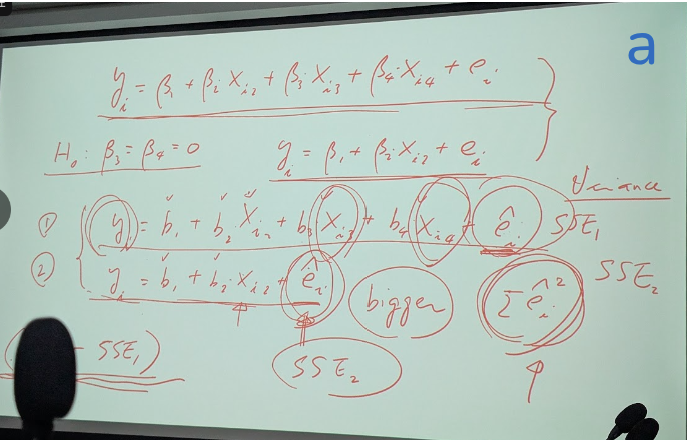
Model(1)&(2): from where? you can see the difference between two model.
b1 b2 .. 難比較,重點是看 e^ (residual) 因為(2)少了xi2 xi3 的idependent variable
所以兩個 e^ 應該會有明顯的差距。觀察、比較這些差距,可以做出推論、判斷。
p問: 常態分配平方加總的機率分配是什麼? 答:就是 卡方分配
(圖b)
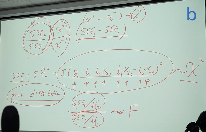
兩個卡方相除 = variance ration = F 就是F 機率分配
如果 (SSE2 - SSE1) 非常大,那表示 xi2 xi3 確是有影響的,也就是 H0: β3 = β4
= 0 可能是要被reject的,但那怎麼知道:這個值是否大到超過呢? 這基準要怎樣訂呢?
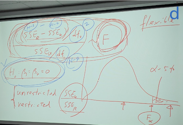
方法是這樣的: 用 (SSE2 - SSE1) / SSE1 ,然而要考慮2和1的樣本數可能各不相同,所以再修訂為 {(SSE2 - SSE1)/df2}
/ {SSE1/df1} ,這就是基準的來源 ~ Fα,df1,df2
model1 叫做 SSEu unrestricted
model2 叫做 SSEr restricted (因為H0: β3 = β4 = 0 變數被限制住了)
所以 {(SSEr - SSEu)/df2} / {SSEu/df1}
這就是F test設計的idea!!!!
df2=(dfr - dfu) = (N-1) -(N-4) = (75-1) -(75-4) = 3
這太好用了 只要run 兩個model 然後比較 SSE就可以判斷了,這就是F的威力,非常好用。被廣泛使用。
-比如你想測 H0: b2=0 本來是用t test, 現在也可以用 F test
(利用比較前後兩個model的SSEu SSEr)
而在這個case中 F = t2
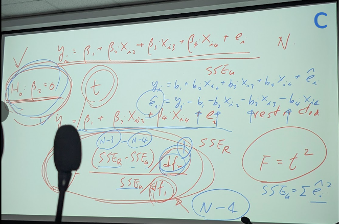
-問df要怎樣算 比如 N-4 怎來的 看(相片c) 有b1..b4 四個綠箭頭 (4 variables?)
df1= dfu = (N- varialbes1) = 75-4 = 71
df2= (dfr - dfu) = (75-2)-(75-4) = 2
接下來我們看例題:(這題重作2025/1204須對課本檢查答案)
p.261 EXAMPLE 6.1 Testing the Effect of Advertising
SSEr = 1896.391 restricted mode (only 2 variable C & b2)
The key is to calculate df1 and df2 first:
(dfu: df unrestricted, dfr: dfrestricted)
df1 = dfu = N-4 = 75-4 = 71
df2 = (dfr - dfu) = (N-2) -(N-4) = (75-2)-(75-4) = 2
= {354.307 / 2} / 21.579
= 177.154 / 21.579 = 8.21
(圖d)
Testing the significent or regression model
this is a default test: 就是假設所有的β等於0 (就是所有idependent variable都沒有時)
你跑軟體時 他會告訴你一個 F值,就是這個(所有的β等於0)
(回歸模型的顯著性檢定-看這模型有沒有必要)
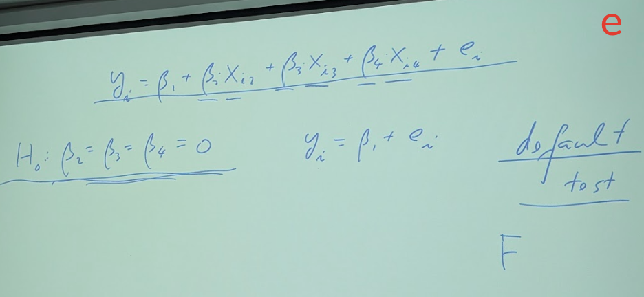
😊During the break, professor asked us to calculate the value of F_default ourselves and see if it matched the result from Eviews: 24.45932.
He gave figure from two models first:
SSEu = 1532.084 unrestricted model (4 variables)
SSEr = 3115.482 restricted mode (only 1 variable C)
The key is to calculate df1 and df2 first:
(dfu: df unrestricted, dfr: dfrestricted)
df1 = dfu = N-4 = 75-4 = 71
df2 = (dfr - dfu) = (N-1) -(N-4) = (75-3)-(75-4) = 3
I calculated it this way. The key is that df1 and df2 cannot be mixed up.
The formula is {(SSEr - SSEu)/df2} / {SSEu/df1}
= {(3115.482 - 1532.084)/3} / {1532.084/71}
= {(1583.398) / 3} / 21.579
= 527.799 / 21.579
= 24.459 Same as the result from Eviews!
你看p.265-EXAMPLE 6.3 Overall Significance of Burger Barns Equation
Big Andy’s Burger Barns 大安迪漢堡店的「獲利方程式」(它在Eviews的資料檔名是andy.wf1)
Equation: SALES = β1 + β2PRICE + β3ADVERT + β4ADVERT2 + e
Hypothesis:
H0∶ β2 = 0, β3 = 0, β4 = 0
H1∶ β2 or β3 or β4 ≠ 0
公式 F = {(SSEr - SSEu)/df2} / {SSEu/df1} = {(SST − SSE)∕(4 − 1)} / {SSE∕(75 − 4)} ∼ F(3,71)
首先,我們可以用Eviews先跑🟢unrestricted的公式(即Model 1):
Quick>Estimate Equation...打入公式>sales c price advert advert^2
得到結果如(圖g)
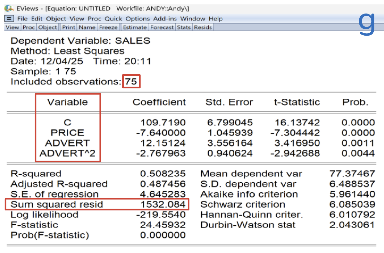
注意: Sum Squared resid就是SSEu (即SSE)=1532.084; 而N是75,變數variable有4個,所以 df1=(N-4)=75-4=71
其次,我們再次用Eviews去跑restricted的公式(即Model 1):
Quick>Estimate Equation...打入公式>sales c
得到結果如(圖h)
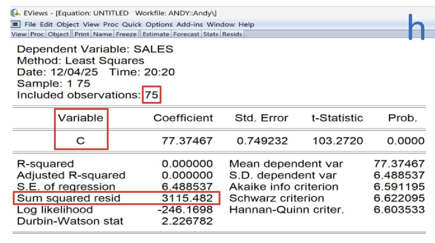
注意: Sum Squared resid就是SSEr (即SST)=3115.482; 而N是75,變數variable只有1個,所以 df2=dfr-dfu=(N-1)-(N-4)=(75-1)-(75-4)=3
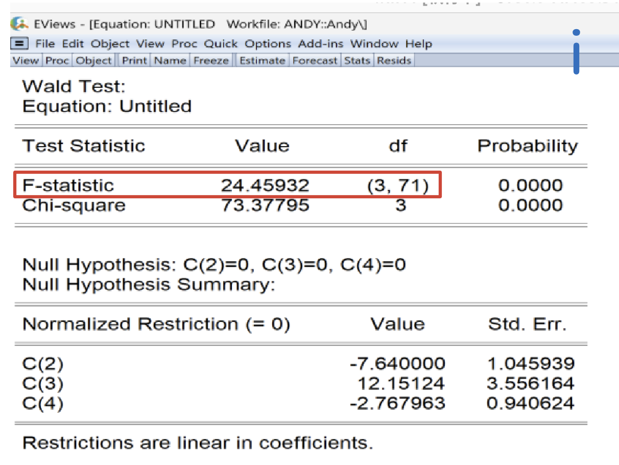
如果要用手算的話,其實就是上面😊During the break, 計算F_default的過程。你看看結果是不是一樣,都是24.459
再來看p.266: EXAMPLE 6.4 When are t- and F-tests equivalent?
Equation(6.9): SALES = β1 + β2PRICE + β3ADVERT + β4ADVERT2 + e
Hypothesis:
H0∶ β2 = 0
H1∶ β2 ≠ 0
公式 F = {(SSEr - SSEu)/df2} / {SSEu/df1} = {(SST − SSE)∕(4 − 3)} / {SSE∕(75 − 4)} ∼ F(1,71)
(跑eviews run equation後再用 Wald Test 設c(2)=0 設第二個係數為0)可算出F= 53.355
在W07有(💡t value)的公式 t= bk / se(bk) ~t(N-2)
Equation: sales c price advert advert^2結果請看(圖g),請注意:β2就是PRICE的係數= -7.640000 而se(Std Error)是 1.045939
根據公式t-value算法是 t = 7.640∕1.045939 = 7.30444
你看: t-value2 =t2=7.304442=53.3548=53.359=F-value
p.267 EXAMPLE 6.5 Testing Optimal Advertising
說: 上週好多同學沒來,這個例題和上週有關,畫(圖f)講解一次: y座標是 TC和TR=Price x Quantity
TC total cost TR total revenue Q是quantity; Profit=TR-TC;
TR是直線 TC是曲線 TC>TR時虧錢
座標下面可以畫出 profit curve
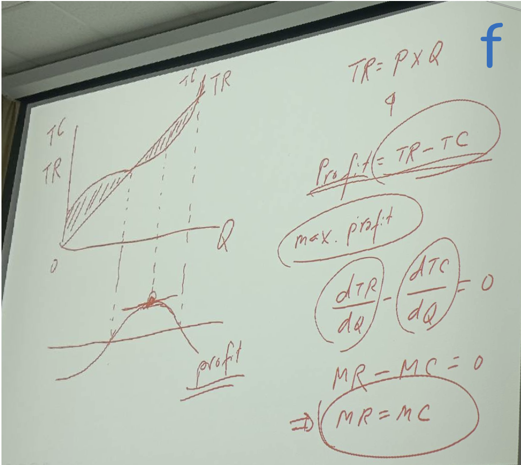
-目標是 max. profit,也就是要找出profit curve 的那個頂點
特性是 斜率為0 (slope of tangent line) 那就是 function的 一階導數 First derivative
就會是 dTR/dQ - dTC/dQ = 0
=MR - MC =marginal revenue - marginal cost = 0
marginal revenue 當你售出additional 1 unit 會得到的revenue,
接下來我們要看Advert(綠字 是一種cost)
在此例中Advert one unit = US$1,000-
(相片): 看怎樣做這個test {β3 + 2β4ADVERT0 = 1 (6.11)}
p.267 EXAMPLE 6.5 Testing Optimal Advertising 只有一個=號,照說用t test也可以,但我們要用F test:
需要回去詳看重作這個 EXAMPLE 6.5
如果你還要做t test, 公式請看相片; 可以自己做做看; wald test表中就有
t value了可比較是否算對
或是像 EXAMPLE 6.6 A One-Tail Test
,老闆可以做各種猜測(假設)員工可用公式算出 假設是否成立!
接下來看p.268 EXAMPLE 6.7 Two (J = 2) Complex Hypotheses 因為有兩個condition 只能用F test
-the conclusion 有三種條件都可能 1不符合 80不符合 或兩者都不符合
再來看p.270但不是太重要 EXAMPLES 6.2 and 6.5 Revisited
要注意EXAMPLE 6.8 A Nonlinear Hypothesis * Optimal condition: Advert0=(1-β3) / 2
β4 怎樣導出來的!
因為H0 是non-lineaing 不好做(公式叫delta method在第五章有介紹過)
然而用Eviews就簡單了
W14 Chapter 6 Further Inference in the Multiple Regression Model
2025-12-10-Tuesday 14:00-17:00 林師模教授
課本: Principles of Econometrics, 5th Edition [P.260] |
講義: Ch-06 Further Inference in the Multiple Regression Model
- 請假(日本仙台旅遊)
- 接著要講:
6.2 The Use of Nonsample Information
6.3 Model Specification
6.4 Prediction (但要skip)
6.5 Poor Data, Collinearity, and Insignificance
6.6 Nonlinear Least Squares
老師想教完第七章.下次應該會講期末報告需要的內容.
W15 Chapter 7 Using Indicator Variables
2025-12-17-Tuesday 14:00-17:00 林師模教授
課本: Principles of Econometrics, 5th Edition [P.317] |
講義: Ch-07 Using Indicator Variables
上週講到p.292的 TAB L E 6.6 Rice Production Function Results from 1994 Data with Constant Returns to Scale
本週從p.294的 6.6 Nonlinear Least Squares 開始講
Those minimizing values are known as the nonlinear least squares estimates.
這本書的focus是linear least square所以不會涉獵太深(不做公式推導只講Eviews怎樣算)
EXAMPLE 6.19 Nonlinear Least Squares Estimates for Simple Model這個沒公式 所以跳過去,講:
EXAMPLE 6.20 A Logistic Growth Curve
討論有個研究是關於Teach Innovation: 當有個new product出現時,market share curve是長這樣的:
S-cureve : logistic curve (圖a)
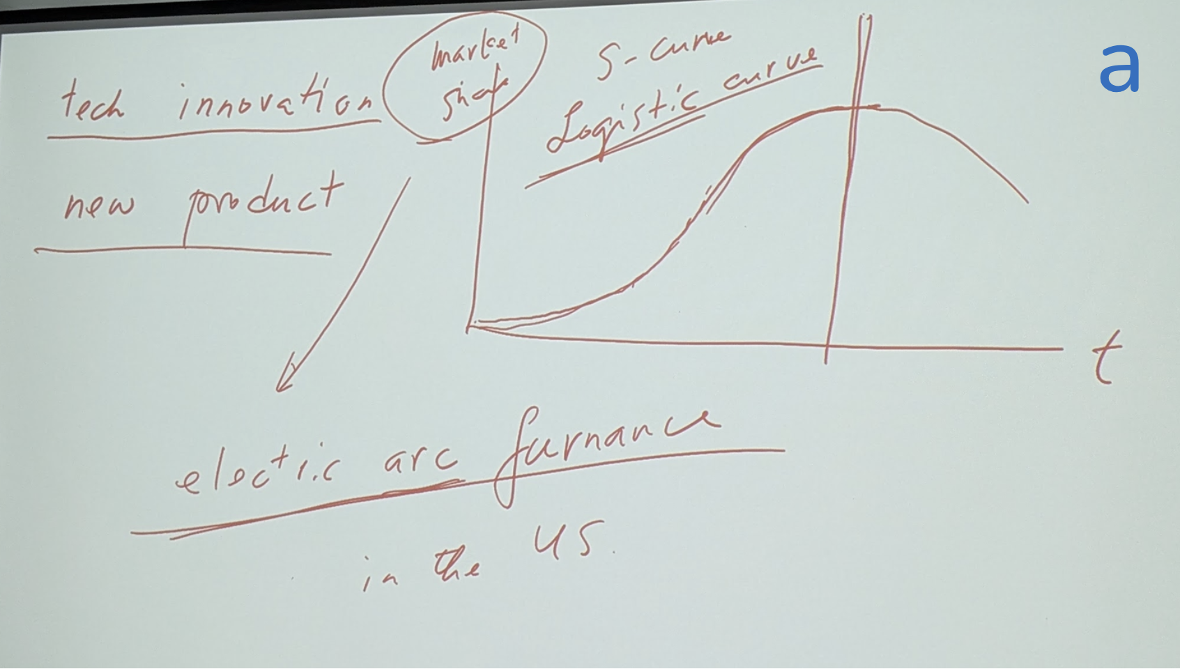
出名的例子就是:高爐煉鋼Blast furnace 轉為電弧爐Electric ark furnace時: market share的變化:
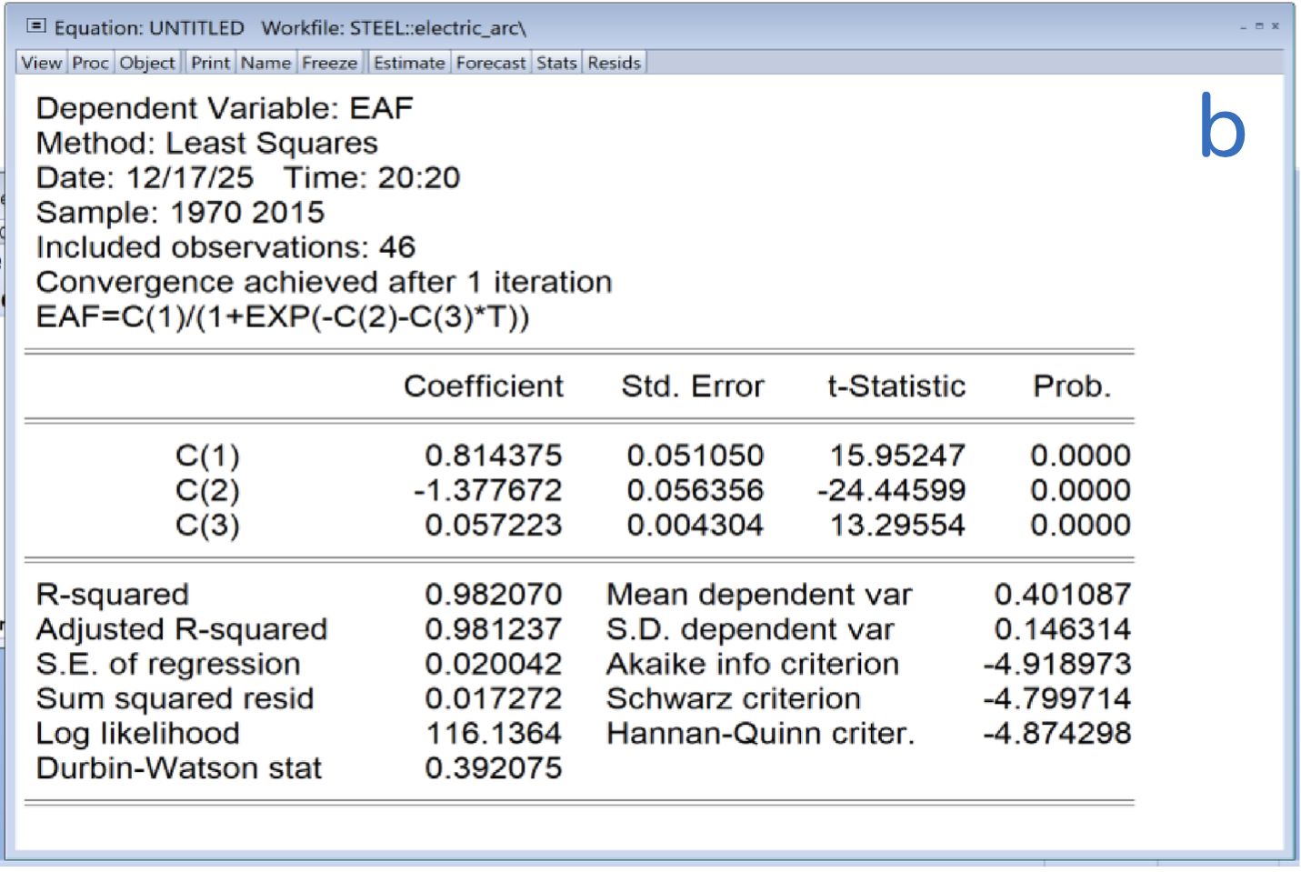
你用Eviews開啟steel.wf1資料檔,會看到 eaf 是Electric ark furnace的縮寫 share 是的市占率是多少(%)的小數點,
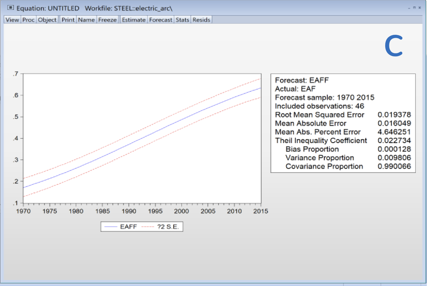
然後run model用 Quick>Estimagte equation> eaf=c(1)/(1+exp(-c(2)-c(3)*t))
(圖b)
還可以進一部做 Focast> eaff (他自動幫你把Focast name設為eaff按下OK就可得圖如下)
(圖c)
用軟體做起來好簡單,這叫「知難行易」:
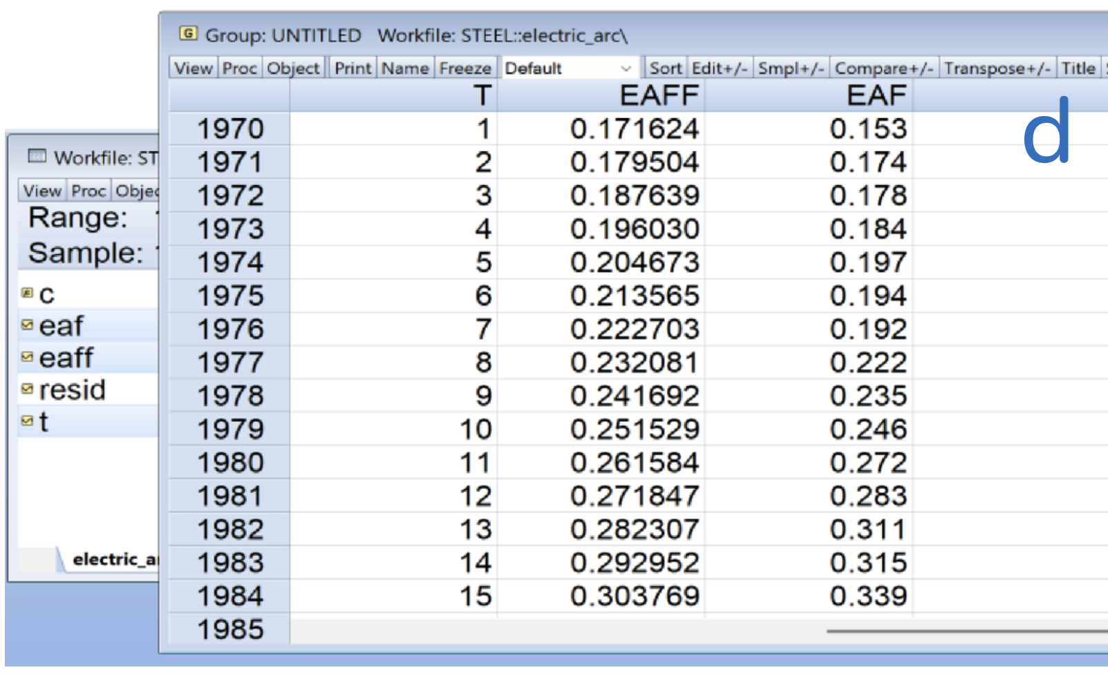
如果要把eaf和eaff疊起來看,可以這樣做:
在steel.wf1先點選t (這是x軸,是independent)然後用Ctl+eaff和Ctl+eaf 選另兩個,然後用右鍵點選Open>as group
(圖d)
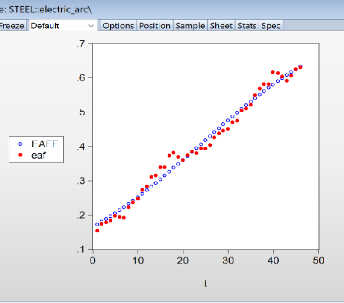
然後再用View > Graph > Scatter 就會畫出這個圖來:(圖e)
Final Report: p.305: 6.22 To examine the quantity theory of money, Brumm15 specifies the equation
deadline: 2026/1/9 submmit the report! no more than 10 pages.
要參考以下Brumm, H.J.(2005)和Moroney J.R.(2002)這兩篇論文:
15-Brumm, H.J. (2005) “Money Growth, Output Growth, and Inflation: A Reexamination of the Modern Quantity Theory’s Linchpin Prediction” Southern Economic Journal, 71(3), 661–667. Paper, | [PDF] |
16-Moroney J.R. (2002), “Money Growth, Output Growth and Inflation: Estimation of a Modern Quantity Theory,” Southern Economic Journal, 69(2), 398–413. Paper | [PDF] |
17-Proving this result requires some advanced calculus. You need to take natural logarithms of both sides, set η = 1 and use l’Hôpital’s rule to take limits as ρ → 0.
W15Final Report | [答案卷] | [PDF] |
2025-12-17三 W1讀完兩篇論文;檢視DataFile: brumm.wf1
2025-12-24三 W2完成報告初稿;
2025-12-31三 W3初稿Revise完成;
2026-01-07三 交卷
接下來開始講 Ch-07 Using Indicator Variables
有6個小節,但7.4 The Linear Probability Model 這節會skip,不講。
在Edition3的第章原名為「非線性關係Nonlinear relationship」在7.2才開始談「虛擬變數Dummy variable」
Ytu What Are Indicator Variables? - The Friendly Statistician.
Ytu Indicator random variables explained in 3 minutes - StatLect official YouTube channel
那要怎樣考慮位置因素,好或不好呢?這是一種「定性因素qualitative factor」, 可以運用二元變數或二分變量,0與1數字(通常稱為虛擬變數,以表示某個特徵是否存在),來進行運算。
加上dummy variable後變成
(7.3)PRICE = β1 + δD + β2SQFT + e
(7.4)E(PRICE | SQFT) = { (β1 + δ ) + β2SQFT 當 D=1
(β1 + β2SQFT 當 D=0 講義錯為 1 了!
看(圖f) 如果run model 會有D=1和 D=0兩條線
(圖f)
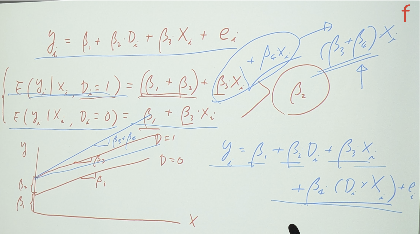
而 β3是一樣的slope,但在事實上,應該是像藍線一樣,會有些差異,那要怎樣modify呢?
方法是在D=1時 再add one more term: interact term
β4(Di * Xi)
這樣藍線的slope就會是 β3+β4 -看(圖f)
-又有時,你收集到的data是靠近加油站等不利因素者,那β4也可能變為負號,那藍線就會偏下方-看(圖f)
老師問 if we slightly chage mode to LD = 0: near 1:not near 也就是反過來設! (原來是0:not near; 1: near; ) ,
那麼兩個model有何不同? (我猜slope不一樣,結果是錯的!) 其實只有intercept不一樣而已。 看(圖g)
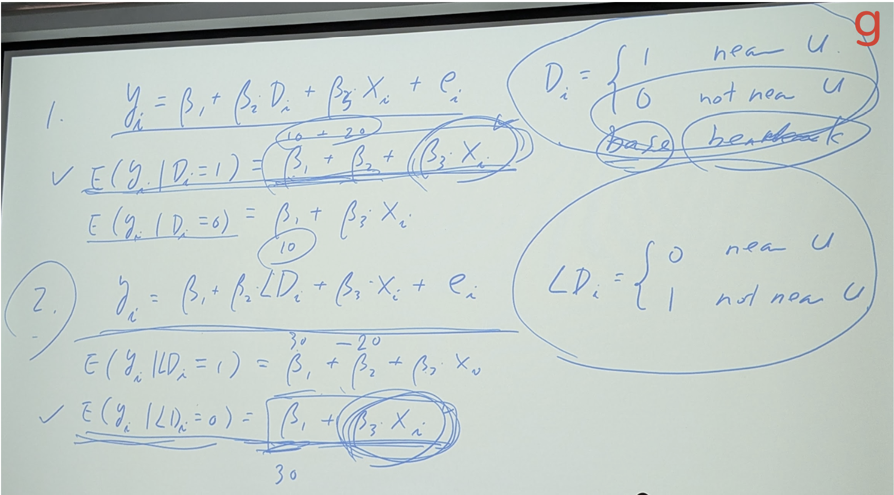
所以有人喜歡D的設法,有人喜歡用LD的設法,其實結果是一樣的,只是係數β1、β2會有變化
注意:通常設為 0 的被稱為Bench mark 至於要那個設為0 是根據你的研究自己來決定。
- 接下來,來看EXAMPLE 7.1 The University Effect on House Prices
UTOWN: 0 not near,1 near university
若用 series LD = 1-utown 這樣就(把0,1的設法)反過來了
兩個同時用不行(看圖h),因為沒意義,因為完全共線性。
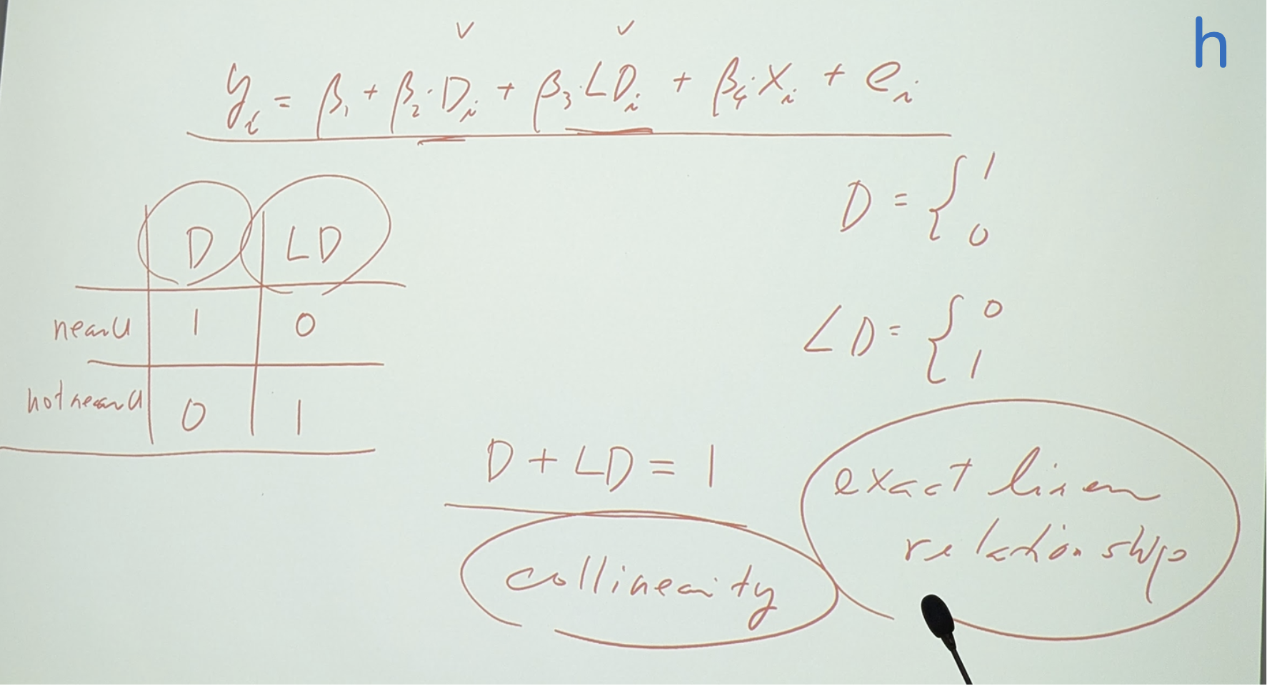
如果兩個變數(D和LD)同時用,那就是個 Dummy Variable Trap。
虛擬變數陷阱Dummy Variable Trap 是指在進行One-Hot Encoding(或虛擬變數編碼)時,生成的虛擬變數之間存在完全多重共線性 的問題。
虛擬變數陷阱(Dummy Variable Trap)是指在進行One-Hot Encoding(或虛擬變數編碼)時,生成的虛擬變數之間存在完全多重共線性 的問題。
1 varialbe 3 cases = 2 dv needs (in, near, not near) (看相片井字格)
Table 7.1,2 pool, fplace 都是dummy variable
根據這個結果,就可做出如下結論
Based on the regression results in Table 7.2, we estimate that
The location premium for lots near the university is $27,453. .....
像− 0.1901AGE 房齡多1價錢會減0.19(*1000元)..
p.323 [7.2.1] Interactions Between Qualitative Factors (Dummy variables)
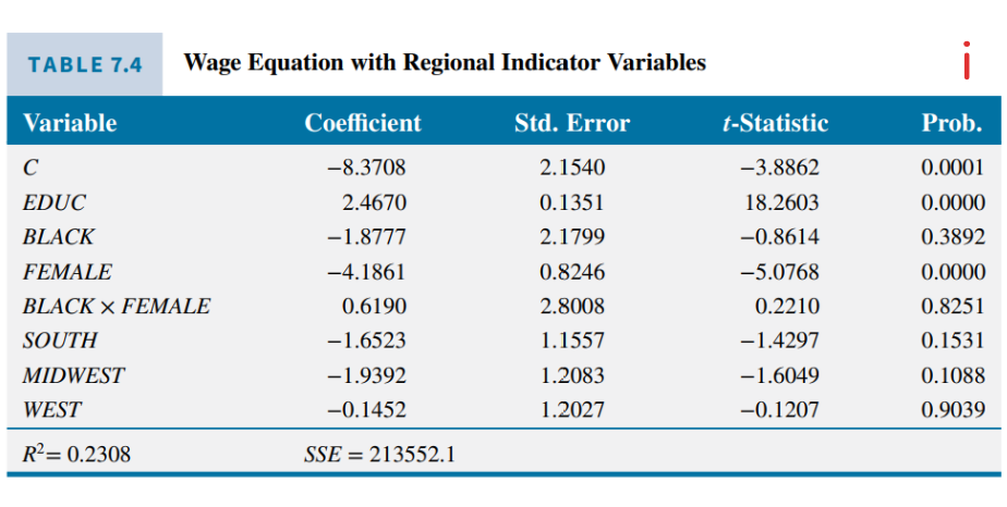
看(7.8) WAGE = β1 + β2EDUC + δ1BLACK + δ2FEMALE + γ(BLACK × FEMALE) + e
δ1,δ2通常都是負數(黑人、女人收入比白人、男人低,是減項),γ期望是正數(回頭做些調整、修正)
這R2很低,因BLACKxFEMALE和 BLACK都not significant
看EXAMPLE 7.2 The Effects of Race and Sex on Wage這個例子
4個cases所以用3個variable 而NORTH作為bench mark
TABLE 7.4 Wage Equation with Regional Indicator Variables 看P-value 有很多insignificant (圖i)
再來談這個 7.2.3 Testing the Equivalence of Two Regressions 就是結構性轉變Structural Change
看(看Sales vs. R&D expd. (圖j)
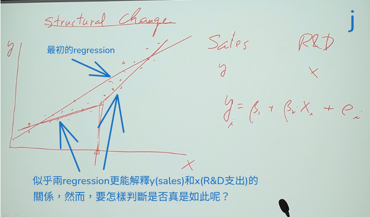
how can we know the twoo regression is better than one regression?
Are two models better than one?
We can perform a "structural change test." If the differences are significant, a bi-regression analysis should be performed; the bilinear model will perform better.
So how should we design the test?
我提議說「可比較slope的差異」,老師說「有3個slope要怎樣設計?有沒有其他的想法?」要怎樣設計 H0: no change?
關鍵是看Residual: 用最初regression的residual,來和(分兩部份的regression 的兩個residual加起來)做比較。看(圖k)
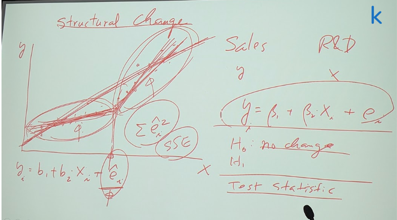
SSER -(SSE1+SSE2) 這個想法 要用F來 設計
注意df的計算方法 :(N-2) - {(N1-2)+(N2-2)} = (N-2)-(N-4) = 2
這個方法是粵裔美國學者鄒至莊發明的,所以被稱做 Chow test (圖L)
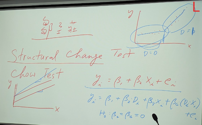
這個test 也可以用 dummy variable來設計:
放個Di 進去 來區分 有沒有(多不多)R&D費用
H0: β2=β4 =0 (看有沒有必要分兩個test 其實就是在看有沒有structural change)
W16 --本週課目標題--
2025-12-24-Tuesday 14:00-17:00 林師模教授
學校放假,不上課!
Final Report: p.305: 6.22 To examine the quantity theory of money, Brumm15 specifies the equation
deadline: 2026/1/9 submmit the report! no more than 10 pages.
要參考以下Brumm, H.J.(2005)和Moroney J.R.(2002)這兩篇論文:
15-Brumm, H.J. (2005) “Money Growth, Output Growth, and Inflation: A Reexamination of the Modern Quantity Theory’s Linchpin Prediction” Southern Economic Journal, 71(3), 661–667. Paper, | [PDF] |
16-Moroney J.R. (2002), “Money Growth, Output Growth and Inflation: Estimation of a Modern Quantity Theory,” Southern Economic Journal, 69(2), 398–413. Paper | [PDF] |
17-Proving this result requires some advanced calculus. You need to take natural logarithms of both sides, set η = 1 and use l’Hôpital’s rule to take limits as ρ → 0.
先複習一下 ▶️ Quantity Theory of Money QTM公式講解 | How Money Supply Drives Inflation 通膨和發鈔數量的關係 With Graphs and Examples |
再研究作業、問題:W15Final Report | [答案卷] | [PDF] |
2025-12-17三 W1讀完兩篇論文;檢視DataFile: brumm.wf1
Part 1: Answer questions a~e using the entire sample (76 countries).
2025/12/21完成Part 1; 接下來要做Part 2,3;
Part 2: Select 40~50 samples and answer questions a~e.
Part 3: Compare the results of Part 1 and Part 2, and explain the reasons for the differences.
**Submit before the end of 1/9. The report should not exceed 10 pages.**
2025-12-31三 W3初稿Revise完成;
2026-01-07三 交卷
W17 --本週課目標題--
2025-12-31-Tuesday 14:00-17:00 林師模教授
課本: Principles of Econometrics, 5th Edition [P.317] |
講義: Ch-07 Using Indicator Variables
- 本學期最後一次上課!
- 前週講到了p.327的EXAMPLE 7.4 | Testing the Equivalence of Two Regressions: The Chow Test
Structural change test
Salesi = β1 + β2 Di + ei 如何判斷 須不需要runing 2 regression, 所以要設計個test to know whether we neet 2 or 1
Can use (SSE1+SSE2) as a Benchmark:
so {SSE -(SSE1+SSE2) /(SSE1+SSE2) } 這樣只是: chi square / chi square ,還是不能做決定
所以,上下要各除以 df 如此一來就變成是 F 了,可以有critical value可用了.
Eviews可以做Chow Test
---也可以用dummy verialbe regression 分開(x)sales小和大兩個group
本節標題就是說 要比較兩個不同的regression
Testing the Equivalence of Two Regressions
The linear probability model - an introduction
The linear probability model - example
The problems with the linear probability model - part 1
The problems with the linear probability model - part 2
The problems with the linear probability model - part 3
Nonlinear discrete choice models - an introduction
線性機率模型 (LPM) 與邏輯斯迴歸 (Logistic Regression)
p.332:Treatment Effects
指特定處理或干預措施(如新藥、政策) 與某結果 (如健康改善、業績提升)之間的因果關係強度。它量化了如果某人接受了處理,與他沒有接受處理相比,結果會有多大的差異,但在實際中無法同時觀察到這兩種「潛在結果」,所以通常用平均處理效果ATE來估計整個人群的平均影響。
- 核心概念
- 潛在結果 Potential Outcomes: 對於每個人,都有兩種可能的結果:一種是接受了處理(例如吃藥),另一種是沒有接受處理(例如吃安慰劑)。
- 個體處理效果 Individual Treatment Effect: 某人接受處理的結果減去未接受處理的結果。
- 平均處理效果 Average Treatment Effect, ATE: 整個群體中所有個體處理效果的平均值,是估計總體因果關係的關鍵指標。 如何測量 (以隨機對照試驗 RCT 為例)
- 隨機分配:將研究對象隨機分成處理組 (接受處理)和對照組 (不接受處理)。
- 比較平均結果:比較處理組的平均結果和對照組的平均結果。
- 估計 ATE: 由於隨機分配確保了兩組在其他方面相似,所以兩組平均結果的差異,就近似於ATE。
為什麼重要
- 區分相關與因果: 幫助我們知道某種干預是否真正導致了結果的改變,而不僅僅是同時發生。
- 政策評估: 評估新政策、教育干預、藥物療效等。
- 個性化推薦: 透過分析異質性處理效果 HTE,了解同一干預對不同特徵群體的差異影響,實現個人化決策。 觀察性研究的挑戰
- 在觀察性研究中(非隨機分配),人們是否接受處理可能受到未觀察因素的影響,這會導致混淆,需要更複雜的統計方法來估計處理效果。
W18 --期末報告--
2026-01-07-Tuesday 14:00-17:00 林師模教授
2026-01-07三 交卷
Q2: 03/13-06/12論文撰寫-2篇JounalPaper投稿/1篇博士論文draft。
Q3: 06/21-09/15大阪-關西外語專門學校-3個月短期課程-目標N2;
Q4: 10/27-28合經同學會; 11/21-29日本萩市;
02資格考phd📚準備
03資格考11,12/菲律賓航行26;
04論文/歷史同學會09-10;
05論文/日本精英會24-29
06論文/台琉杯帆賽06-13/日本16,21
07日本 大阪-關西外語專門學校-短期班6/15-9/15
08日本
09日本
10合經同學會27-28
11萩市21-29
Backup Data 其他參考資料
Book | Data Miming | Data Science for Business |
URL | Kaggle | 彭明輝教授
1.演講Youtube: 期刊論文閱讀技巧
2.演講Youtube: 研究生的核心能力 ─ 從文獻回顧到批判與創新 │Future Faculty Talk
▼1 WHAT IS INFORMATION MANAGEMENT?
WHAT IS INFORMATION MANAGEMENT?
1.ANIMATION FOR PLATONWHAT IS INFORMATION MANAGEMENT? wearesynkro 2014。2. Information Management BasicsCommunity IT Innovators 2018。
3.(IM) Information Management JuanIT 2021。有一系列lecture
4.The 5 Components of an Information System COTC A.R.C. 2015。
▼2 自習課程-Ben Lambert、Bob、李宗璋老師
自習課程-Ben Lambert、Bob、李宗璋老師
牛津大學 Ben Lambert Econometrics | 筆記 | 李柏堅 CUSTcourses |【Mandarin國語】五分鐘計量經濟學(計量經濟學輔導)
第一集:什麼是OLS?
第二集:什麼是因果效應?
第三集:什麼是擬合值與殘差?
第四集:什麼是OLS擬合值與殘差的特點?
第五集:什麼是普通最小方差估計量的無偏特點? 第六集:什麼是高斯馬可夫定理?
第七集:什麼是“Ceteris Paribus”?
第八集:什麼是“零條件期望假定”和“零相關假定”?
第九集:什麼是SST,SSE,和SSR?
第十集:什麼是F統計量和F檢驗?
第十一集:什麼是R-squared和Adjusted R-squared?
第十二集:Stata回歸結果窗口有哪些統計量?
第十三集:什麼是遺留變量偏差?
第十四集:怎樣減緩遺留變量偏差?
第十五集:什麼是Frisch-Waugh-Lovell (FWL)定理?
第十六集:計量經濟模型與理論經濟模型的區別是什麼?
第十七集:如何描述對數變量和水平變量的系數估計值?
第十八集:經典線性模型的六個假設是什麼?
第十九集:什麼是內生解釋變量和外生解釋變量?Endogenous and exogenous explanatory variables
(phd19_Chapter 10 Endogenous Regressors and Moment-Based Estimation 隨機解釋變數撼動差估計)
第二十集:什麼是迴歸模型的矩陣表達形式?
第二十一集:如何推導矩陣形式的OLS估計量?什麼是投影矩陣和殘差生成矩陣?
第二十二集:如何推導OLS估計量(使用代數和矩陣)?
第二十三集:多元變量模型OLS估計量什麼時候跟部分模型OLS估計量相同?
第二十四集:什麼是矩陣的基礎概念和特點?
Economics in Real Life (Episode 5)
Episode 1 Income Inequality and Gini Coefficient
Episode 2 Game Theory and Prisoner’s Dilemma
Episode 3 Economic Development as Freedom
Episode 4 The Nature of Poverty
Episode 5 Tragedy of the Commons and the Overuse of Public Resources
Episode 6 Is A Bumper Harvest Always Good for Farmers?
Episode 7 Eviews 2 导入EXCEL文件
3.Eviews 3 绘制散点图
4.Eviews 4 估计回归方程
5.Eviews 5 主菜单简介
6.Eviews 6 series的操作
7.Eviews 7 group的操作
8.Eviews 8 equation的操作
9.Eviews 9 Jarque Bera test
10.Eviews 10 输出结果数值显示格式的设置
11.Eviews 11 多元回归
12.Eviews 12 受限最小二乘
13.Eviews 13 完全共线性
14.Eviews 14 多项式双对数倒数模型
15.Eviews 15 单个序列的绘图命令
16.Eviews 16 两个序列的绘图命令
17.Eviews 17 回归模型的命令
18.Eviews 18 虚拟变量的引入
19.Eviews 19 虚拟变量的交互项
20.Eviews 20 季节分析中的虚拟变量
21.Eviews 21 遗漏或多余变量的检验
22.Eviews 22 reset检验
23.eviews 23 多重共线性
24.Eviews 24 残差的图形诊断
25.Eviews 25 异方差检验
26.Eviews 26 加权最小二乘
27.Eviews 27 怀特异方差校正值
28.Eviews 28 自相关的图形诊断
29.Eviews 29 自相关LM检验
30.Eviews 30 广义差分变化
31.Eviews 31 Neway West校正值
32.如何使用Excel高级筛选工具?
EViews 14